
The first MATH6014 test will be held at 5 p.m. today. The test is worth 15% of your final mark. The test will be 50 minutes long and you must answer all questions. Question 3 is worth 40 marks; Questions 1 and 2 30 marks each. I will put the formula for the roots of a quadratic equation on the paper. Please find a sample here.
I am emailing a link of this to everyone on the class list every week. If you are not receiving these emails or want to have them sent to another email address feel free to email me at jippo@campus.ie and I will add you to the mailing list.
This Week
We developed our applications of step and impulse functions to beam equations. Relevant notes p.22 – 50
In the tutorial we worked on the sample test.
Next Week
We have a tutorial on Thursday. Please take this opportunity to nail down the differential equations. On the final exam there will be both a full question on beam equations and a full question on second order linear differential equations. Hence if you are comfortable with the material that is examinable in the test, feel free to move onto some of the exercises on beam equations.
![]()
Test Date
Tuesday 13 March at 6.45 p.m.
Timetable Changes
We are now going to schedule ourselves as follows:
Week 6: – & Tutorial
Week 7: Lecture/Test & –
Week 8: Lecture & Lecture
Week 9: Tutorial & Lecture
Week 10: Tutorial & Lecture
Week 11: – & Lecture
Week 12: Tutorial & Lecture
Sample Test Answers
Here I give you links to how I checked answers quickly using Wolfram Alpha. It takes Mathematica code (they are the same company) and will probably decipher your own stab at code also. Note that Wolfram Alpha gives us a lot more information than we need but that is the beauty of the thing really.
Question 1 — note there is a small typo here it should be 
Question 2 — it’s not evaluating the constants using the boundary conditions for some reason… the answer is
Question 4 — the boundary conditions yield 
Question 5 — what is 

Question 6 — again we need to realise that the notation here is different to ours. Applying the boundary conditions we get ![y(x)=3[x-8]^3-3[x-2]^3+54x](https://s0.wp.com/latex.php?latex=y%28x%29%3D3%5Bx-8%5D%5E3-3%5Bx-2%5D%5E3%2B54x&bg=ffffff&fg=545454&s=0&c=20201002)
I am emailing a link of this to everyone on the class list every week. If you are not receiving these emails or want to have them sent to another email address feel free to email me at jippo@campus.ie and I will add you to the mailing list.
This Week
We looked at different types of data and how to present them. Notes here. When we look at histograms next week this section will be complete. In Maple we continued to boost our basic skills and looked at Maple’s LinearAlgebra package.
Next Week
I hope to finish looking at histograms. Then we will begin our study of probability, asking the question what is a random variable and when are random variables independent?
Reminder
The test will be held at 7.05 p.m. sharp on Wednesday 14 March.
Sample Test Answers
Here I give you links to how I checked answers quickly using Wolfram Alpha. It takes Mathematica code (they are the same company) and will probably decipher Maple code too (moreover Maple code with ‘adjustments’). Note that Wolfram Alpha gives us a lot more information than we need but that is the beauty of the thing really.
Question 1 (has a slight typo: should be 
Question 3 — this implies that there are non-trivial solutions. Now that we know that it has non-trivial (non-zero solutions) so we can use Wolfram Alpha to solve for these (in terms of a parameter 

Bonus Questions
You could do without all the notation. The underlined would do.
1. Firstly the linear system can be written as a set of simultaneous equations:


The solution set is not changed by 


2. 
3. You can solve the system for one rather than all variables.
In this section we introduce the important GNS construction and prove that every C*-algebra can be regarded as a C*-subalgebra of 

A representation of a C*-algebra 


The Question
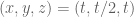
The pressure, volume, and temperature of an ideal gas are related by the equation 

Solution
First of all, solving for 
Now we can go further and say that both 

![P(T(t),V(t))=\frac{8.31T(t)}{V(t)}=8.31T(t)[V(t)]^{-1}](https://s0.wp.com/latex.php?latex=P%28T%28t%29%2CV%28t%29%29%3D%5Cfrac%7B8.31T%28t%29%7D%7BV%28t%29%7D%3D8.31T%28t%29%5BV%28t%29%5D%5E%7B-1%7D&bg=ffffff&fg=545454&s=0&c=20201002)
I am emailing a link of this to everyone on the class list every week. If you are not receiving these emails or want to have them sent to another email address feel free to email me at jippo@campus.ie and I will add you to the mailing list.
This Week
We said that a homogeneous linear system was one where all the constants are zero. We then proved the following:
Proposition
Let 


- If
then the system has (an infinite number of) non-trivial solutions.
- If
then the system has (a unique solution given by) the trivial solution (
).
Consider this notice for the test on Wednesday 14 March at 7 p.m (Wednesday fortnight).
Please find a sample test here.
I am emailing a link of this to everyone on the class list every week. If you are not receiving these emails or want to have them sent to another email address feel free to email me at jippo@campus.ie and I will add you to the mailing list.
This Week
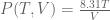
We introduced step and impulse functions to model loads on a beam and we wrote down the equations relating the loading, the shearing force, the bending moment and the deflection. Relevant notes p.23 to p.43.
In the tutorial we worked on the exercises on second order linear differential equations in these notes.
Next Week
We have a tutorial on Tuesday. In this we will try to shore up the second order differential equations and the second order differential equations involving step and impulse functions. Remember the integration of impulse and step functions is given by (where each of the arrows indicate an integration)
![\delta(x-a)\rightarrow H(x-a)\rightarrow [x-a]\rightarrow\frac{[x-a]^2}{2}](https://s0.wp.com/latex.php?latex=%5Cdelta%28x-a%29%5Crightarrow+H%28x-a%29%5Crightarrow+%5Bx-a%5D%5Crightarrow%5Cfrac%7B%5Bx-a%5D%5E2%7D%7B2%7D&bg=ffffff&fg=545454&s=0&c=20201002)
![\int [x-a]^n\,dx=\frac{[x-a]^{n+1}}{n+1}](https://s0.wp.com/latex.php?latex=%5Cint+%5Bx-a%5D%5En%5C%2Cdx%3D%5Cfrac%7B%5Bx-a%5D%5E%7Bn%2B1%7D%7D%7Bn%2B1%7D&bg=ffffff&fg=545454&s=0&c=20201002)
Also each integration generates an addition constant 
In next weeks lectures we will continue our work on the beam equations.
Consider this notice for the test on Tuesday 13 March at 6.45 p.m (just under three weeks away) (note that there is still a small chance that this tell will be held on Thursday 8 March at 8.15 p.m.).
Please find a sample test here
Note that the format will be the same as this.
- Homogeneous Second Order Linear
- Homogeneous Second Order Linear with boundary/initial conditions
- Non-Homogeneous Second Order Linear
- Non-Homogeneous Second Order Linear with boundary/initial conditions
- Second Order Separable with Step and Impulse Functions
- Second Order Separable with Step and Impulse Functions with boundary/initial conditions
Q. 5 and 6 will be covered Thursday night. Note that for questions 1-4 the roots will not be complex — although they could be fractions or surds (i.e. ye might need the 
For abelian C*-algebras we were able to completely determine the structure of the algebra in terms of the character space, that is, in terms of the one-dimensional representations. For the non-abelian case this is quite inadequate, and we have to look at representations of arbitrary dimension. There is a deep inter-relationship between the representations and the positive linear functionals of a C*-algebra. Representations will be defined and some aspects of this inter-relationship investigated in the next section. In this section we establish the basis properties of positive linear functionals.

Recent Comments