
You are currently browsing the category archive for the ‘MATH6028’ category.
A Poker Hack
I told this story in class on Friday. I wasn’t sure if it was true but it appears that it is.
Texas Hold’Em Poker
‘Texas‘ is a poker game where a number of players sit around a table. Two cards are dealt to each player. There after follows a round of betting, the reveal of three more cards (the flop), more betting, another card (the turn), another round of betting, another card (the river), and another round of betting:

What we are interested in is what happens after all this, before another hand is dealt?
The deck is shuffled.
A shuffle is required to mix up the deck. Here we used three terms: deck, shuffle, mixed up. These can all be given a precise mathematical realisation (see the introduction here for more). Mixed up means ‘close to random’. Here let me introduce a mathematical realisation of random:
If one is handed a deck of cards, face down, and if each possible order of
the cards is equally possible then the deck is considered random.
Note there are 

One popular method of shuffling cards is the riffle shuffle. In a remarkable 1992 paper by Bayer & Diaconis, with a really cool name: Trailing the Dovetail Shuffle to Its Lair, it is shown that seven riffle shuffles are necessary and sufficient to get a deck close to random:

Here we see 


So the idea is after, say, ten shuffles (or, equivalently, about ten rounds of hands), the deck is mixed up or close to random: each of the 52! orders are approximately likely.
The Fibonacci Sequence is given by the recursive definition:
Exercises
- Prove that if
satisfies the recurrence relation

that 
- If the Fibonacci Sequence is given by:

where 


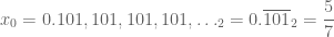
- Use ten terms of the Fibonacci Sequence to write down a sequence of rational approximations to
.
- Using
.
This follows on from this post.
Recall the Doubling Mapping 

At the end of the last post we showed that this dynamical system displays sensitivity to initial conditions. Now we show that it displays topological mixing (a chaotic orbit) and density of periodic points.
First we must talk about periodic points.
Periodic Points
Consider, for example, the initial state 

Here we see 
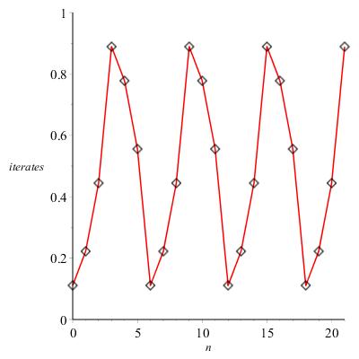
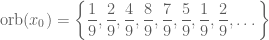
The orbit of 
The orbit of any fraction, e.g. 


and there are only 243 of these and so after 244 iterations, some state must be repeated and so we get locked into a periodic cycle.
If we accept the following:
Proposition
A fraction 

then this is another way to see that fractions are (eventually) periodic. Take for example,
Geometric Series
Let 


Therefore the sequence is given by:
Such a sequence is called a geometric sequence with common ratio 
When we add up the terms a sequence we have a geometric sum:

Here 
We can find a formula for


Exercises
Assuming that 

Binary Numbers
Exercises
- Write the following as fractions:

- Use infinite geometric series to show that:


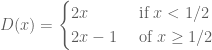
Doubling Mapping
The doubling mapping
Exercises
- Find the first six iterates of the point
under
.
- Find the first four iterates of the point

- Where
has the binary representation

write down expressions for 

- Hence find points
such that
and
agree to 5 binary digits but
and
differ in the first binary digit for some
.
- Describe the period-5 points of
- Let
have a binary representation beginning
. Find a period-5 point
of
and
- Find a
such that there are iterates of
,
, with
, that agree with 0.111 , 0.101, and 0.010, to three binary
digits.
Sensitivity to Initial Conditions
Exercise
Let 
![[0,1]](https://s0.wp.com/latex.php?latex=%5B0%2C1%5D&bg=ffffff&fg=545454&s=0&c=20201002)
![f:[0,1]\rightarrow [0,1]](https://s0.wp.com/latex.php?latex=f%3A%5B0%2C1%5D%5Crightarrow+%5B0%2C1%5D&bg=ffffff&fg=545454&s=0&c=20201002)


Dynamical Systems
A dynamical system is a set of states 


and in general, the next state is got by applying the iterator function:

The sequence of states
is known as the orbit of 
Such dynamical systems are completely deterministic: if you know the state at any time you know it at all subsequent times. Also, if a state is repeated, for example:

then the orbit is destined to repeated forever because


Example: Savings
Suppose you save in a bank, where monthly you receive 

This can be modeled as a dynamical system.
Let 


Now, in the second month, there is interest on all this:
interest in second month 
we also have the 

and it shouldn’t be too difficult to see that how you get from 

Exercise
Use geometric series to find a formula for 
Weather
If quantum effects are neglected, then weather is a deterministic system. This means that if we know the exact state of the weather at a certain instant (we can even think of the state of the universe – variations in the sun affecting the weather, etc), then we can calculate the state of the weather at all subsequent times.
This means that if we know everything about the state of the weather today at 12 noon, then we know what the weather will be at 12 noon tomorrow…

Recent Comments