
You are currently browsing the category archive for the ‘General’ category.
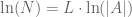
This is just a little exercise in partial differentiation
Introduction
So, you have a password of length 


In this sense we will assume that passwords are subject only to random guesses, and so we make the simple assumption that given the data 
The set of passwords is 

Simple Numerics
A simple approach is to simply make a table:
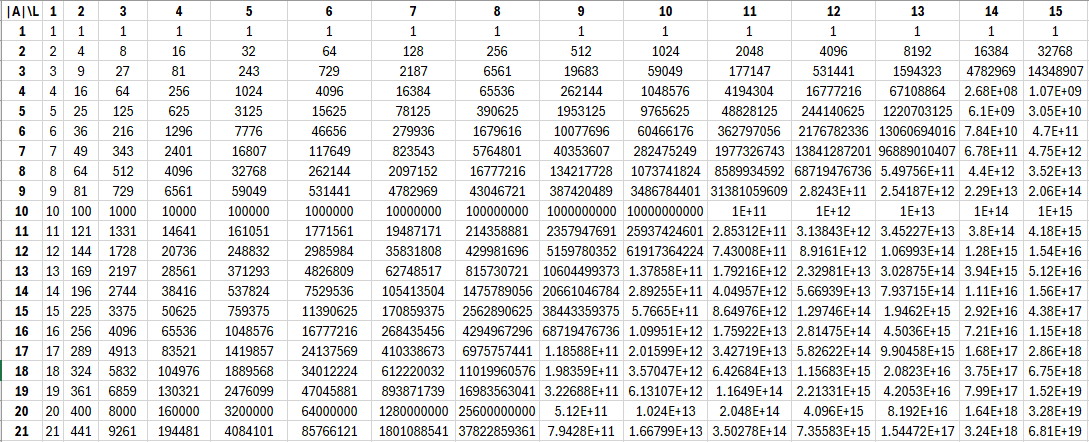
An eyeballing of this will tell you that most of time it appears that increasing the length is preferable to increasing the alphabet size. But then again, alphabet size jumps tend to be larger, e.g. 26 to 52, 52 to 62, etc.
Suppose you have a length 


Some analysis
Consider a password from a set of 
- increase the alphabet size:
, or
- increase the password length
.
If we look what these do to the number of passwords:
vs
,
we are comparing 


For example, from the table above, at 


But for a fixed 
So, if you have a length 61 password from an alphabet of size 20, you are better off increasing the alphabet size.
I guess what is relevant here are the following questions: at 
- If
, and
.
- If
, you could increase the length of the password rather than jumping to
.
- If
, you could increase the length of the password rather than jumping to
.
Going to special characters only makes sense in our framework if there is also a password length condition of 10 or more.
Partial Differentiation
This wasn’t even what I wanted to do here, which was to approximate this question using partial differentiation. In all these questions we are asking about what happens to 


Even I can differentiate with respect to

We might use some logs to differentiate with respect to


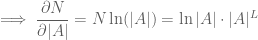
These partial derivatives estimate that if 


so, approximately, we are left comparing 


Alice, Bob and Carol are hanging around, messing with playing cards.
Alice and Bob each have a new deck of cards, and Alice, Bob, and Carol all know what order the decks are in.
Carol has to go away for a few hours.
Alice starts shuffling the deck of cards with the following weird shuffle: she selects two (different) cards at random, and swaps them. She does this for hours, doing it hundreds and hundreds of times.
Bob does the same with his deck.
Carol comes back and asked “have you mixed up those decks yet?” A deck of cards is “mixed up” if each possible order is approximately equally likely:
![\displaystyle \mathbb{P}[\text{ deck in order }\sigma\in S_{52}]\approx \frac{1}{52!}](https://s0.wp.com/latex.php?latex=%5Cdisplaystyle+%5Cmathbb%7BP%7D%5B%5Ctext%7B+deck+in+order+%7D%5Csigma%5Cin+S_%7B52%7D%5D%5Capprox+%5Cfrac%7B1%7D%7B52%21%7D&bg=ffffff&fg=545454&s=0&c=20201002)
She asks Alice how many times she shuffled the deck. Alice says she doesn’t know, but it was hundreds, nay thousands of times. Carol says, great, your deck is mixed up!
Bob pipes up and says “I don’t know how many times I shuffled either. But I am fairly sure it was over a thousand”. Carol was just about to say, great job mixing up the deck, when Bob interjects “I do know that I did an even number of shuffles though.“.
Why does this mean that Bob’s deck isn’t mixed up?
I am not sure has the following observation been made:
When the Jacobi Method is used to approximate the solution of Laplace’s Equation, if the initial temperature distribution is given by
, then the iterations
are also approximations to the solution,
, of the Heat Equation, assuming the initial temperature distribution is
I first considered such a thought while looking at approximations to the solution of Laplace’s Equation on a thin plate. The way I implemented the approximations was I wrote the iterations onto an Excel worksheet, and also included conditional formatting to represent the areas of hotter and colder, and the following kind of output was produced:
Let me say before I go on that this was an implementation of the Gauss-Seidel Method rather than the Jacobi Method, and furthermore the stopping rule used was the rather crude 
However, do not the iterations resemble the flow of heat from the heat source on the bottom through the plate? The aim of this post is to investigate this further. All boundaries will be assumed uninsulated to ease analysis.
Discretisation
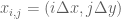
Consider a thin rod of length 


Suppose are interested in the temperature of the rod at a point ![x\in[0,L]](https://s0.wp.com/latex.php?latex=x%5Cin%5B0%2CL%5D&bg=ffffff&fg=545454&s=0&c=20201002)


Similarly we can mesh a plate of dimensions 


![\mathbf{x}\in[0,W]\times [0,H]](https://s0.wp.com/latex.php?latex=%5Cmathbf%7Bx%7D%5Cin%5B0%2CW%5D%5Ctimes+%5B0%2CH%5D&bg=ffffff&fg=545454&s=0&c=20201002)


We can also mesh a box of dimension 


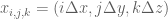
![\mathbf{x}\in [0,W]\times [0,D]\times [0,H]](https://s0.wp.com/latex.php?latex=%5Cmathbf%7Bx%7D%5Cin+%5B0%2CW%5D%5Ctimes+%5B0%2CD%5D%5Ctimes+%5B0%2CH%5D&bg=ffffff&fg=545454&s=0&c=20201002)


Finite Differences
How the temperature evolves is given by partial differential equations, expressing relationships between
We are the mathematicians and they are the physicists (all jibes and swipes are to be taken lightly!!)
A
A is for atom and axiom. While we build beautiful universes from our carefully considered axioms, they try and destroy this one by smashing atoms together.
B
B is for the Banach-Tarski Paradox, proof if it was ever needed that the imaginary worlds which we construct are far more interesting then the dullard of a one that they study.
C
C is for Calculus and Cauchy. They gave us calculus about 340 years ago: it only took us about 140 years to make sure it wasn’t all nonsense! Thanks Cauchy!
D
D is for Dimension. First they said there were three, then Einstein said four, and now it ranges from 6 to 11 to 24 depending on the day of the week. No such problems for us: we just use
E
E is for Error Terms. We control them, optimise them, upper bound them… they just pretend they’re equal to zero.
F
F is for Fundamental Theorems… they don’t have any.
G
G is for Gravity and Geometry. Ye were great yeah when that apple fell on Newton’s head however it was us asking stupid questions about parallel lines that allowed Einstein to formulate his epic theory of General Relativity.
H
H is for Hole as in the Black Hole they are going to create at CERN.
I
I is for Infinity. In the hand of us a beautiful concept — in the hands of you an ugliness to be swept under the carpet via the euphemism of “renormalisation”…
J
J is for Jerk: the third derivative of displacement. Did you know that the fourth, fifth, and sixth derivatives are known as Snap, Crackle, and Pop? No, I did not know they had a sense of humour either.
K
K is for Knot Theory. A mathematician meets an experimental physicist in a bar and they start talking.
- Physicist: “What kind of math do you do?”,
- Mathematician: “Knot theory.”
- Physicist: “Yeah, Me neither!”
L
L is for Lasers. I genuinely spent half an hour online looking for a joke, or a pun, or something humorous about lasers… Lost Ample Seconds: Exhausting, Regrettable Search.
M
M is for Mathematical Physics: a halfway house for those who lack the imagination for mathematics and the recklessness for physics.
N
N is for the Nobel Prize, of which many mathematicians have won, but never in mathematics of course. Only one physicist has won the Fields Medal.
O
O is for Optics. Optics are great: can’t knock em… 7 years bad luck.
P
P is for Power Series. There are rules about wielding power series; rules that, if broken, give gibberish such as the sum of the natural numbers being 
Q
Q is for Quark… they named them after a line in Joyce as the theory makes about as much sense as Joyce.
R
R is for Relativity. They are relatively pleasant.
S
S is for Singularities… instead of saying “we’re stuck” they say “singularity”.
T
T is for Tarksi… Tarski had a son called Jon who was a physicist. Tarksi always appears twice.
U
U is for the Uncertainty Principle. I am uncertain as to whether writing this was a good idea.
V
V is for Vacuum… Did you hear about the physicist who wanted to sell his vacuum cleaner? Yeah… it was just gathering dust.
W
W is for the Many-Worlds-Interpretation of Quantum Physics, according to which, Mayo GAA lose All-Ireland Finals in infinitely many different ways.
X
X is unknown.
Y
Y is for Yucky. Definition: messy or disgusting. Example: Their “Calculations”
Z
Z is for Particle Zoo… their theories are getting out of control. They started with atoms and indeed atoms are only the start. Pandora’s Box has nothing on these people.. forget baryons, bosons, mesons, and quarks: the latest theories ask for sneutrinos and squarks; photinos and gluinos, zynos and even winos. A zoo indeed.
PS
We didn’t even mention String Theory!
The End.
A colleague writes (extract):
“I have an assessment with 4 sections in it A,B,C and D.
I have a question bank for each section. The number of questions in each bank is A-10, B-10, C-5, D-5.
In my assessment I will print out randomly a fixed number of questions from each bank. Section A will have 5 questions, B-5, C-2, D-2. 14 questions in total appear on the exam.
I can figure out how many different exam papers (order doesn’t matter) can be generated (I think!).
But my question is: what is the uniqueness of each exam, or what overlap between exams can be expected.?
I am not trying to get unique exams for everyone (unique as in no identical questions) but would kinda like to know what is the overlap.“

Following the same argument as here we can establish that:
Fact 1
The expected number of students to share an exam is 
Let the number of exams 
This is an approach that takes advantage of the fact that expectation is linear, and the probability of an event 
![\displaystyle\mathbb{P}[\text{not-}E]=1-\mathbb{P}[E]](https://s0.wp.com/latex.php?latex=%5Cdisplaystyle%5Cmathbb%7BP%7D%5B%5Ctext%7Bnot-%7DE%5D%3D1-%5Cmathbb%7BP%7D%5BE%5D&bg=ffffff&fg=545454&s=0&c=20201002)
Label the 20 students by 


Then 

and we can calculate, using the linearity of expectation.
![\mathbb{E}[X]=\mathbb{E}[S_1]+\cdots \mathbb{E}[S_{20}]](https://s0.wp.com/latex.php?latex=%5Cmathbb%7BE%7D%5BX%5D%3D%5Cmathbb%7BE%7D%5BS_1%5D%2B%5Ccdots+%5Cmathbb%7BE%7D%5BS_%7B20%7D%5D&bg=ffffff&fg=545454&s=0&c=20201002)
The 

![\displaystyle\mathbb{E}[S_i]=0\times\mathbb{P}[S_i=0]+1\times \mathbb{P}[S_i=1]](https://s0.wp.com/latex.php?latex=%5Cdisplaystyle%5Cmathbb%7BE%7D%5BS_i%5D%3D0%5Ctimes%5Cmathbb%7BP%7D%5BS_i%3D0%5D%2B1%5Ctimes+%5Cmathbb%7BP%7D%5BS_i%3D1%5D&bg=ffffff&fg=545454&s=0&c=20201002)
but ![\displaystyle\mathbb{P}[S_i=0]=\mathbb{P}[\text{ student i does not share an exam}]=p](https://s0.wp.com/latex.php?latex=%5Cdisplaystyle%5Cmathbb%7BP%7D%5BS_i%3D0%5D%3D%5Cmathbb%7BP%7D%5B%5Ctext%7B+student+i+does+not+share+an+exam%7D%5D%3Dp&bg=ffffff&fg=545454&s=0&c=20201002)
![\displaystyle \mathbb{P}[S_i=1]=\mathbb{P}[\text{not-}(S_i=0)]=1-\mathbb{P}[S_i=0]=1-p](https://s0.wp.com/latex.php?latex=%5Cdisplaystyle+%5Cmathbb%7BP%7D%5BS_i%3D1%5D%3D%5Cmathbb%7BP%7D%5B%5Ctext%7Bnot-%7D%28S_i%3D0%29%5D%3D1-%5Cmathbb%7BP%7D%5BS_i%3D0%5D%3D1-p&bg=ffffff&fg=545454&s=0&c=20201002)
and so
![\displaystyle\mathbb{E}[S_i]=1-p](https://s0.wp.com/latex.php?latex=%5Cdisplaystyle%5Cmathbb%7BE%7D%5BS_i%5D%3D1-p&bg=ffffff&fg=545454&s=0&c=20201002)
All of the 20
![\displaystyle\mathbb{E}[X]=20\cdot (1-p)](https://s0.wp.com/latex.php?latex=%5Cdisplaystyle%5Cmathbb%7BE%7D%5BX%5D%3D20%5Ccdot+%281-p%29&bg=ffffff&fg=545454&s=0&c=20201002)
Now, what is the probability that nobody shares student
We need students 


![\mathbb{P}[\text{(student j not sharing) AND (student k not sharing)}]](https://s0.wp.com/latex.php?latex=%5Cmathbb%7BP%7D%5B%5Ctext%7B%28student+j+not+sharing%29+AND+%28student+k+not+sharing%29%7D%5D&bg=ffffff&fg=545454&s=0&c=20201002)
So we have that

and so the answer to the question is:
![\displaystyle\mathbb{E}[X]=20\cdot \left(1-\left(\frac{\alpha-1}{\alpha}\right)^{19}\right)\approx 0.00005985\approx 0.00006](https://s0.wp.com/latex.php?latex=%5Cdisplaystyle%5Cmathbb%7BE%7D%5BX%5D%3D20%5Ccdot+%5Cleft%281-%5Cleft%28%5Cfrac%7B%5Calpha-1%7D%7B%5Calpha%7D%5Cright%29%5E%7B19%7D%5Cright%29%5Capprox+0.00005985%5Capprox+0.00006&bg=ffffff&fg=545454&s=0&c=20201002)
We can get an estimate for the probability that two or more students share an exam using Markov’s Inequality:
![\displaystyle\mathbb{P}[X\geq 2]\leq \frac{\mathbb{E}[X]}{2}\approx 0.00003=0.003\%](https://s0.wp.com/latex.php?latex=%5Cdisplaystyle%5Cmathbb%7BP%7D%5BX%5Cgeq+2%5D%5Cleq+%5Cfrac%7B%5Cmathbb%7BE%7D%5BX%5D%7D%7B2%7D%5Capprox+0.00003%3D0.003%5C%25&bg=ffffff&fg=545454&s=0&c=20201002)
Fact 2
This estimate is tight: the probability that two or more students (out of 20) share an exam is about 0.003%.
This tallies very well with the exact probability which can be found using a standard Birthday Problem argument (see the solution to Q. 7 here) to be:
![\mathbb{P}[X\geq 2]\approx 0.0000299191\approx 0.003\%](https://s0.wp.com/latex.php?latex=%5Cmathbb%7BP%7D%5BX%5Cgeq+2%5D%5Capprox+0.0000299191%5Capprox+0.003%5C%25&bg=ffffff&fg=545454&s=0&c=20201002)
The probability that two given students share an exam is

Fact 3
The expected number of shared questions between two students is 6.6
Take students 1 and 2. The questions are in four bins: two of ten, two of five. Let 

![\displaystyle \mathbb{E}[Q]=\sum_{i=1}^4\mathbb{E}[B_i]](https://s0.wp.com/latex.php?latex=%5Cdisplaystyle+%5Cmathbb%7BE%7D%5BQ%5D%3D%5Csum_%7Bi%3D1%7D%5E4%5Cmathbb%7BE%7D%5BB_i%5D&bg=ffffff&fg=545454&s=0&c=20201002)
and the numbers are small enough to calculate the probabilities exactly using the hypergeometric distribution.
The calculations for bins 1 and 2, and bins 3 and 4 are the same. The expectation
![\displaystyle\mathbb{E}[B_1]=\sum_{j=0}^5j\mathbb{P}[B_1=j]](https://s0.wp.com/latex.php?latex=%5Cdisplaystyle%5Cmathbb%7BE%7D%5BB_1%5D%3D%5Csum_%7Bj%3D0%7D%5E5j%5Cmathbb%7BP%7D%5BB_1%3Dj%5D&bg=ffffff&fg=545454&s=0&c=20201002)
Writing briefly ![p_j=\mathbb{P}[B_1=j]](https://s0.wp.com/latex.php?latex=p_j%3D%5Cmathbb%7BP%7D%5BB_1%3Dj%5D&bg=ffffff&fg=545454&s=0&c=20201002)

and we find:
![\displaystyle\mathbb{E}[B_1]=\mathbb{E}[B_2]=\frac52](https://s0.wp.com/latex.php?latex=%5Cdisplaystyle%5Cmathbb%7BE%7D%5BB_1%5D%3D%5Cmathbb%7BE%7D%5BB_2%5D%3D%5Cfrac52&bg=ffffff&fg=545454&s=0&c=20201002)
Similarly we see that
![\displaystyle\mathbb{E}[B_3]=\mathbb{E}[B_4]=\frac{4}{5}](https://s0.wp.com/latex.php?latex=%5Cdisplaystyle%5Cmathbb%7BE%7D%5BB_3%5D%3D%5Cmathbb%7BE%7D%5BB_4%5D%3D%5Cfrac%7B4%7D%7B5%7D&bg=ffffff&fg=545454&s=0&c=20201002)
and so, using linearity:
![\displaystyle\mathbb{E}[Q]=\frac52+\frac52+\frac45+\frac45=6.6](https://s0.wp.com/latex.php?latex=%5Cdisplaystyle%5Cmathbb%7BE%7D%5BQ%5D%3D%5Cfrac52%2B%5Cfrac52%2B%5Cfrac45%2B%5Cfrac45%3D6.6&bg=ffffff&fg=545454&s=0&c=20201002)
This suggests that on average students share about 50% of the question paper. Markov’s Inequality gives:
![\displaystyle\mathbb{P}[Q\geq 7]\underset{\approx}{\leq} 0.9429](https://s0.wp.com/latex.php?latex=%5Cdisplaystyle%5Cmathbb%7BP%7D%5BQ%5Cgeq+7%5D%5Cunderset%7B%5Capprox%7D%7B%5Cleq%7D+0.9429&bg=ffffff&fg=545454&s=0&c=20201002)
but I do not believe this is tight.
Calculating this probability exactly is tricky because there are many different ways that students can share a certain number of questions. We would be looking at something like “multiple hypergeometric”, and I would calculate it as the event not-(0 or 1 or 2 or 3 or 4 or 5 or 6).
I think the ![\mathbb{E}[Q]=6.6](https://s0.wp.com/latex.php?latex=%5Cmathbb%7BE%7D%5BQ%5D%3D6.6&bg=ffffff&fg=545454&s=0&c=20201002)
We tell four tales of De Morgan.
In each case we have something that looks like AND, something that looks like OR, and something that looks like NOT.
Sets
The Collection of Objects
Consider a universe of discourse/universal set/ambient set 


The collection of objects in this case is the set of subsets of 
Suppose, for the purposes of illustration, that
Consider the subsets 

in the obvious way.
AND
Note that two objects are contained both in 

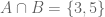
We can represent the ambient set
We can demonstrate for a general
Slides of a talk given at CIT School of Science Seminar.
Talk delivered to the Conversations on Teaching and Learning Winter Programme 2018/19, organised by the Teaching & Learning Unit in CIT (click link for slides):
Contexts and Concepts: A Case Study of Mathematics Assessment for Civil & Environmental Engineering
I received the following email (extract) from a colleague:
With the birthday question the chances of 23 people having unique birthdays is less than ½ so probability of shared birthdays is greater than 1-in-2.
Coincidentally on the day you sent out the paper, the following question/math fact was in my son’s 5th Class homework.
We are still debating the answer, hopefully you could clarify…
In a group of 368 people, how many should share the same birthday. There are 16×23 in 368 so there are 16 ways that 2 people should share same birthday (?) but my son pointed out, what about 3 people or 4 people etc.
I don’t think this is an easy problem at all.
First off we assume nobody is born on a leap day and the distribution of birthdays is uniform among the 365 possible birthdays. We also assume the birthdays are independent (so no twins and such).
They were probably going for 16 or 32 but that is wrong both for the reasons given by your son but also for the fact that people in different sets of 23 can also share birthdays.
The brute force way of calculating it is to call by
![\displaystyle \mathbb{E}[X]=\sum_{i=2}^{368}i\cdot \mathbb{P}[X=i]](https://s0.wp.com/latex.php?latex=%5Cdisplaystyle+%5Cmathbb%7BE%7D%5BX%5D%3D%5Csum_%7Bi%3D2%7D%5E%7B368%7Di%5Ccdot+%5Cmathbb%7BP%7D%5BX%3Di%5D&bg=ffffff&fg=545454&s=0&c=20201002)
Already we have that ![\mathbb{P}[X=2]=\mathbb{P}[X=3]=0](https://s0.wp.com/latex.php?latex=%5Cmathbb%7BP%7D%5BX%3D2%5D%3D%5Cmathbb%7BP%7D%5BX%3D3%5D%3D0&bg=ffffff&fg=545454&s=0&c=20201002)
![\mathbb{P}[X=4]](https://s0.wp.com/latex.php?latex=%5Cmathbb%7BP%7D%5BX%3D4%5D&bg=ffffff&fg=545454&s=0&c=20201002)

For 
- 5 share a birthday, 363 different birthdays, OR
- 2 share a birthday, 3 share a different birthday, and the remaining 363 have different birthdays
Then 
- 6 share a birthday, 362 different birthdays, OR
- 3, 3, 362
- 4, 2, 362
- 2, 2, 2, 362
This problem is spiraling out of control.
There is another approach that takes advantage of the fact that expectation is linear, and the probability of an event
Label the 368 people by 

Then

and we can calculate, using the linearity of expectation.
![\mathbb{E}[X]=\mathbb{E}[S_1]+\cdots \mathbb{E}[S_{368}]](https://s0.wp.com/latex.php?latex=%5Cmathbb%7BE%7D%5BX%5D%3D%5Cmathbb%7BE%7D%5BS_1%5D%2B%5Ccdots+%5Cmathbb%7BE%7D%5BS_%7B368%7D%5D&bg=ffffff&fg=545454&s=0&c=20201002)
The
but ![\displaystyle\mathbb{P}[S_i=0]=\mathbb{P}[\text{ person i does not share a birthday}]=p](https://s0.wp.com/latex.php?latex=%5Cdisplaystyle%5Cmathbb%7BP%7D%5BS_i%3D0%5D%3D%5Cmathbb%7BP%7D%5B%5Ctext%7B+person+i+does+not+share+a+birthday%7D%5D%3Dp&bg=ffffff&fg=545454&s=0&c=20201002)
and so
All of the 368
![\displaystyle\mathbb{E}[X]=368\cdot (1-p)](https://s0.wp.com/latex.php?latex=%5Cdisplaystyle%5Cmathbb%7BE%7D%5BX%5D%3D368%5Ccdot+%281-p%29&bg=ffffff&fg=545454&s=0&c=20201002)
Now, what is the probability that nobody shares person
We need persons 
![\mathbb{P}[\text{(person k not sharing) AND (person k not sharing)}]](https://s0.wp.com/latex.php?latex=%5Cmathbb%7BP%7D%5B%5Ctext%7B%28person+k+not+sharing%29+AND+%28person+k+not+sharing%29%7D%5D&bg=ffffff&fg=545454&s=0&c=20201002)
So we have that

and so the answer to the question is:
![\displaystyle\mathbb{E}[X]=368\cdot \left(1-\left(\frac{364}{365}\right)^{367}\right)\approx 233.54\approx 234](https://s0.wp.com/latex.php?latex=%5Cdisplaystyle%5Cmathbb%7BE%7D%5BX%5D%3D368%5Ccdot+%5Cleft%281-%5Cleft%28%5Cfrac%7B364%7D%7B365%7D%5Cright%29%5E%7B367%7D%5Cright%29%5Capprox+233.54%5Capprox+234&bg=ffffff&fg=545454&s=0&c=20201002)
There is possibly another way of answering this using the fact that with 368 people there are
pairs of people.
This strategy is by no means optimal nor exhaustive. It is for students who are struggling with basic integration and anti-differentiation and need something to help them start calculating straightforward integrals and finding anti-derivatives.
TL;DR: The strategy to antidifferentiate a function 
- Direct
- Manipulation
-Substitution
- Parts

Recent Comments