
You are currently browsing the category archive for the ‘Probability Theory’ category.
Consider the symmetric group 


![X\sim \mathrm{Poi}[1]](https://s0.wp.com/latex.php?latex=X%5Csim+%5Cmathrm%7BPoi%7D%5B1%5D&bg=ffffff&fg=545454&s=0&c=20201002)


![\displaystyle \lim_{N\to \infty}\mathbb{P}[\mathrm{fix}_N(\xi_N)=m]=\mathbb{P}[X=m]](https://s0.wp.com/latex.php?latex=%5Cdisplaystyle+%5Clim_%7BN%5Cto+%5Cinfty%7D%5Cmathbb%7BP%7D%5B%5Cmathrm%7Bfix%7D_N%28%5Cxi_N%29%3Dm%5D%3D%5Cmathbb%7BP%7D%5BX%3Dm%5D&bg=ffffff&fg=545454&s=0&c=20201002)
In this note we will look at the distribution in the case where the uniform distribution is conditioned on 
Theorem
Let ![1+\mathrm{Poi}[1]](https://s0.wp.com/latex.php?latex=1%2B%5Cmathrm%7BPoi%7D%5B1%5D&bg=ffffff&fg=545454&s=0&c=20201002)
![\displaystyle \lim_{N\to \infty}\mathbb{P}[\mathrm{fix}_N(\xi_N)=m]=\mathbb{P}[X=m-1]](https://s0.wp.com/latex.php?latex=%5Cdisplaystyle+%5Clim_%7BN%5Cto+%5Cinfty%7D%5Cmathbb%7BP%7D%5B%5Cmathrm%7Bfix%7D_N%28%5Cxi_N%29%3Dm%5D%3D%5Cmathbb%7BP%7D%5BX%3Dm-1%5D&bg=ffffff&fg=545454&s=0&c=20201002)
Proof: What can be shown, ostensibly from stuff from the quantum permutation side of the house is that, where 


the 

![\displaystyle \sum_{t=0}^\infty t^k\mathbb{P}[1+X=t]=\sum_{t=0}^\infty t^k\mathbb{P}[X=t-1]](https://s0.wp.com/latex.php?latex=%5Cdisplaystyle+%5Csum_%7Bt%3D0%7D%5E%5Cinfty+t%5Ek%5Cmathbb%7BP%7D%5B1%2BX%3Dt%5D%3D%5Csum_%7Bt%3D0%7D%5E%5Cinfty+t%5Ek%5Cmathbb%7BP%7D%5BX%3Dt-1%5D&bg=ffffff&fg=545454&s=0&c=20201002)


using the fact that the Bell numbers are the moments of that Poisson distribution and the standard recurrence for the Bell numbers.
Local vs Global Conditioning of Quantum Permutations
In the quantum case we define

where 


Note that when we measure the Haar state with some finite spectrum version of
- the probability of finding an integer number of fixed points is zero, and
- independently of
, the probability of finding more than four fixed points is zero.
In the classical case above when we chose the permutation uniformly from those who fix one, there are two ways of viewing it:
- we pick an element of
- we consider the isotropy subgroup
and choose our permutation from
.
Classically, these are the same thing. In the quantum case these two things can be interpreted differently. The second case is quite clear in the quantum case. For 


The analogue of the uniform distribution on 


I guess this is marginally more interesting than the unshifted version.
Now, what about an analogue of “we pick an element of 

And, it turns out, as above, using stuff from the quantum permutation side of the house:
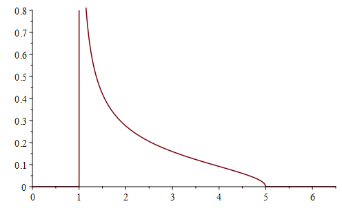
Quite quickly from here we find that the density of the distribution of 

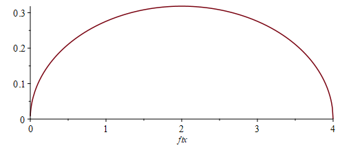
This is so interesting:
- it doesn’t change the support — we still find between 0 and 4 fixed points,
- we have a new symmetry about
, we had another unexpected symmetry here.
- the mean jumps from one to two, that is not unexpected, but
- the mode jumps from zero to two!
- even though we have observed one to one, there can still be less than one fixed point when we measure… and this happens with probability
.
The next obvious question is what happens with:

Epilogue?
So what about this local vs global conditioning? Well, no matter what subsequent measurements are made to
This is not the case with
Classical Warm-up
Let 

This algebra is commutative, but we will use some non-commutative algebraic analogues. Let 


When choosing a permutation at random what is the probability that it sends 
![\displaystyle \mathbb{P}[\pi(1)=1]=\pi(\mathbf{1}_{1\to 1})=\frac{1}{N}](https://s0.wp.com/latex.php?latex=%5Cdisplaystyle+%5Cmathbb%7BP%7D%5B%5Cpi%281%29%3D1%5D%3D%5Cpi%28%5Cmathbf%7B1%7D_%7B1%5Cto+1%7D%29%3D%5Cfrac%7B1%7D%7BN%7D&bg=ffffff&fg=545454&s=0&c=20201002)
Once this has been observed, there is a conditioning of the state 

The state was given by 
Consider a subset 

This is an observable, which basically asks of a permutation, do you map three into 
What is the probability that a random permutation maps three into
We find, with a fairly elementary calculation that the answer to this question is:
![\displaystyle \mathbb{P}[\pi_{1\to 1}(3)\in S]=\frac{|S|}{N-1}](https://s0.wp.com/latex.php?latex=%5Cdisplaystyle+%5Cmathbb%7BP%7D%5B%5Cpi_%7B1%5Cto+1%7D%283%29%5Cin+S%5D%3D%5Cfrac%7B%7CS%7C%7D%7BN-1%7D&bg=ffffff&fg=545454&s=0&c=20201002)
If 


What is the probability that after seeing 

![\displaystyle \mathbb{P}[\nu(2)=2]=\frac{1}{N-2}](https://s0.wp.com/latex.php?latex=%5Cdisplaystyle+%5Cmathbb%7BP%7D%5B%5Cnu%282%29%3D2%5D%3D%5Cfrac%7B1%7D%7BN-2%7D&bg=ffffff&fg=545454&s=0&c=20201002)
Therefore, where 
![\displaystyle \mathbb{P}[(\pi(2)=2)\succ (\pi(3)\in S)\succ(\pi(1)=1)]](https://s0.wp.com/latex.php?latex=%5Cdisplaystyle+%5Cmathbb%7BP%7D%5B%28%5Cpi%282%29%3D2%29%5Csucc+%28%5Cpi%283%29%5Cin+S%29%5Csucc%28%5Cpi%281%29%3D1%29%5D&bg=ffffff&fg=545454&s=0&c=20201002)

Now let us ask a ridiculous question. What was the probability that 
![\displaystyle \mathbb{P}[\pi_{1\to 1}(1)=1]=\dfrac{\pi(\mathbf{1}_{1\to 1}\mathbf{1}_{1\to 1}\mathbf{1}_{1\to 1})}{\pi(\mathbf{1}_{1\to 1})}=1](https://s0.wp.com/latex.php?latex=%5Cdisplaystyle+%5Cmathbb%7BP%7D%5B%5Cpi_%7B1%5Cto+1%7D%281%29%3D1%5D%3D%5Cdfrac%7B%5Cpi%28%5Cmathbf%7B1%7D_%7B1%5Cto+1%7D%5Cmathbf%7B1%7D_%7B1%5Cto+1%7D%5Cmathbf%7B1%7D_%7B1%5Cto+1%7D%29%7D%7B%5Cpi%28%5Cmathbf%7B1%7D_%7B1%5Cto+1%7D%29%7D%3D1&bg=ffffff&fg=545454&s=0&c=20201002)
Of course the answer is zero. Can we actually see it in the above framework: well, yes, because the algebra of functions is commutative. You end up with evaluating a state at

but commutativity sees 

We don’t have to do state conditioning and multiplication to calculate the probability that a random permutation maps one to one, then maps three into 

Let us remark that this probability is increasing in 

Let’s Go Quantum
In the case of quantum permutations, so talking 


![\displaystyle \mathbb{P}[(h(1)=2)\succ(h(3)=3)\succ (h(1=1))]=\frac{N-3}{q(N)}](https://s0.wp.com/latex.php?latex=%5Cdisplaystyle+%5Cmathbb%7BP%7D%5B%28h%281%29%3D2%29%5Csucc%28h%283%29%3D3%29%5Csucc+%28h%281%3D1%29%29%5D%3D%5Cfrac%7BN-3%7D%7Bq%28N%29%7D&bg=ffffff&fg=545454&s=0&c=20201002)
Anyway, the quantum versions of the 

![\mathbb{P}[(h(2)=2)\succ (h(3)\in S)\succ (h(1)=1)]:=h(|u_{22}u_{S,3}u_{11}|^2)](https://s0.wp.com/latex.php?latex=%5Cmathbb%7BP%7D%5B%28h%282%29%3D2%29%5Csucc+%28h%283%29%5Cin+S%29%5Csucc+%28h%281%29%3D1%29%5D%3A%3Dh%28%7Cu_%7B22%7Du_%7BS%2C3%7Du_%7B11%7D%7C%5E2%29&bg=ffffff&fg=545454&s=0&c=20201002)
where 
![\displaystyle \mathbb{P}[(h(2)=2)\succ (h(3)\in S)\succ (h(1)=1)]=\frac{|S|(N^2-5N+5+|S|)}{(N-2)q(N)}](https://s0.wp.com/latex.php?latex=%5Cdisplaystyle+%5Cmathbb%7BP%7D%5B%28h%282%29%3D2%29%5Csucc+%28h%283%29%5Cin+S%29%5Csucc+%28h%281%29%3D1%29%5D%3D%5Cfrac%7B%7CS%7C%28N%5E2-5N%2B5%2B%7CS%7C%29%7D%7B%28N-2%29q%28N%29%7D&bg=ffffff&fg=545454&s=0&c=20201002)
This is also increasing in 
This quantity is related to the classical probability above, and there are asymptotic similarities. Writing 


![\displaystyle \mathbb{P}[(h(2)=2)\succ (h(3)\in S)\succ (h(1)=1)]](https://s0.wp.com/latex.php?latex=%5Cdisplaystyle+%5Cmathbb%7BP%7D%5B%28h%282%29%3D2%29%5Csucc+%28h%283%29%5Cin+S%29%5Csucc+%28h%281%29%3D1%29%5D&bg=ffffff&fg=545454&s=0&c=20201002)
![\displaystyle=\mathbb{P}[(\pi(2)=2)\succ (\pi(3)\in S)\succ(\pi(1)=1)]\cdot\left[1-\frac{|S^c|+1}{q(N)}\right]](https://s0.wp.com/latex.php?latex=%5Cdisplaystyle%3D%5Cmathbb%7BP%7D%5B%28%5Cpi%282%29%3D2%29%5Csucc+%28%5Cpi%283%29%5Cin+S%29%5Csucc%28%5Cpi%281%29%3D1%29%5D%5Ccdot%5Cleft%5B1-%5Cfrac%7B%7CS%5Ec%7C%2B1%7D%7Bq%28N%29%7D%5Cright%5D&bg=ffffff&fg=545454&s=0&c=20201002)
I guess this also says, the larger
A twist
What if instead of looking at 


From our classical intuition, we would probably just expect, well, the same really. The larger the value of 


![\displaystyle \mathbb{P}[(h(1)=2)\succ (h(3)\in S)\succ (h(1)=1)]=\dfrac{|S|(N-2-|S|)}{q(N)}](https://s0.wp.com/latex.php?latex=%5Cdisplaystyle+%5Cmathbb%7BP%7D%5B%28h%281%29%3D2%29%5Csucc+%28h%283%29%5Cin+S%29%5Csucc+%28h%281%29%3D1%29%5D%3D%5Cdfrac%7B%7CS%7C%28N-2-%7CS%7C%29%7D%7Bq%28N%29%7D&bg=ffffff&fg=545454&s=0&c=20201002)
Proof: Consider 


Like in the classical case, by definition here, 

Now, classically, this is just a sum of zero terms equal to zero, but not in the quantum world where we have these 

Now take the 

This yields the strange probability above. I think any intuition I have for this would be very much post-hoc. I think I will just let it hang there as something weird, cool and mysterious about quantum permutations…
Alice, Bob and Carol are hanging around, messing with playing cards.
Alice and Bob each have a new deck of cards, and Alice, Bob, and Carol all know what order the decks are in.
Carol has to go away for a few hours.
Alice starts shuffling the deck of cards with the following weird shuffle: she selects two (different) cards at random, and swaps them. She does this for hours, doing it hundreds and hundreds of times.
Bob does the same with his deck.
Carol comes back and asked “have you mixed up those decks yet?” A deck of cards is “mixed up” if each possible order is approximately equally likely:
![\displaystyle \mathbb{P}[\text{ deck in order }\sigma\in S_{52}]\approx \frac{1}{52!}](https://s0.wp.com/latex.php?latex=%5Cdisplaystyle+%5Cmathbb%7BP%7D%5B%5Ctext%7B+deck+in+order+%7D%5Csigma%5Cin+S_%7B52%7D%5D%5Capprox+%5Cfrac%7B1%7D%7B52%21%7D&bg=ffffff&fg=545454&s=0&c=20201002)
She asks Alice how many times she shuffled the deck. Alice says she doesn’t know, but it was hundreds, nay thousands of times. Carol says, great, your deck is mixed up!
Bob pipes up and says “I don’t know how many times I shuffled either. But I am fairly sure it was over a thousand”. Carol was just about to say, great job mixing up the deck, when Bob interjects “I do know that I did an even number of shuffles though.“.
Why does this mean that Bob’s deck isn’t mixed up?
Abstract
Necessary and sufficient conditions for a Markov chain to be ergodic are that the chain is irreducible and aperiodic. This result is manifest in the case of random walks on finite groups by a statement about the support of the driving probability: a random walk on a finite group is ergodic if and only if the support is not concentrated on a proper subgroup, nor on a coset of a proper normal subgroup. The study of random walks on finite groups extends naturally to the study of random walks on finite quantum groups, where a state on the algebra of functions plays the role of the driving probability. Necessary and sufficient conditions for ergodicity of a random walk on a finite quantum group are given on the support projection of the driving state.
Link to journal here.
In my pursuit of an Ergodic Theorem for Random Walks on (probably finite) Quantum Groups, I have been looking at analogues of Irreducible and Periodic. I have, more or less, got a handle on irreducibility, but I am better at periodicity than aperiodicity.
The question of how to generalise these notions from the (finite) classical to noncommutative world has already been considered in a paper (whose title is the title of this post) of Fagnola and Pellicer. I can use their definition of periodic, and show that the definition of irreducible that I use is equivalent. This post is based largely on that paper.
Introduction
Consider a random walk on a finite group 


The convolution is also implemented by right multiplication by the stochastic operator:

where 


and so the stochastic operator 
The random walk driven by 


![[P^k]_{1\ell}>0](https://s0.wp.com/latex.php?latex=%5BP%5Ek%5D_%7B1%5Cell%7D%3E0&bg=ffffff&fg=545454&s=0&c=20201002)
The period of the random walk is defined by:
![\displaystyle \gcd\left(d\in\mathbb{N}:[P^d]_{11}>0\right)](https://s0.wp.com/latex.php?latex=%5Cdisplaystyle+%5Cgcd%5Cleft%28d%5Cin%5Cmathbb%7BN%7D%3A%5BP%5Ed%5D_%7B11%7D%3E0%5Cright%29&bg=ffffff&fg=545454&s=0&c=20201002)
The random walk is said to be aperiodic if the period of the random walk is one.
These statements have counterparts on the set level.
If 
Moreover, when 


In fact, in this case it is necessarily the case that 


Suppose that 


This shows how the stochastic operator reduces the index
A central component of Fagnola and Pellicer’s paper are results about how the decomposition of a stochastic operator:

specifically the maps 
Stochastic Operators and Operator Algebras
Let 


It can be shown that if 

All hereditary subalgebras are of this form.
In a recent preprint, Haonan Zhang shows that if 


The algebra of functions 

As it happens, where 


To help with intuition, making the incorrect assumption that 

as for classical groups 
That is the condition 
Consider a random walk on a classical (the algebra of functions on
The following is a very non-algebra-of-functions-y proof that 
Proof: Let 

We claim that the random walk on
The driving probability
If 

Therefore,

Apart from the big reason — that this proof talks about points galore — this kind of proof is not available in the quantum case because there exist
So we have some questions:
- Is there a proof of the classical result (above) in the language of the algebra of functions on
- And can this proof be adapted to the quantum case?
- Is the claim perhaps true for all finite quantum groups but not all compact quantum groups?
Quantum Subgroups
Let 


The Classical Case
In the classical case, where the algebras of functions on

There is a natural embedding, in the classical case, if 

with 


Furthermore,

which resembles 
In the case where
where the i.i.d. 

We can also prove this using the language of the commutative algebra of functions on

Consider now two probabilities on 


Consider


that is 
Some Questions
Back to quantum groups with non-commutative algebras of functions.
- Can we embed
and do we have
, giving the projection-like quality to
- Is
a suitable definition for
If this is the case, the above proof carries through to the quantum case.
- If there is no such embedding, what is the appropriate definition of a
- If
Edit
UwF has recommended that I look at this paper to improve my understanding of the concepts involved.
Slides of a talk given at the Irish Mathematical Society 2018 Meeting at University College Dublin, August 2018.
Abstract Four generalisations are used to illustrate the topic. The generalisation from finite “classical” groups to finite quantum groups is motivated using the language of functors (“classical” in this context meaning that the algebra of functions on the group is commutative). The generalisation from random walks on finite “classical” groups to random walks on finite quantum groups is given, as is the generalisation of total variation distance to the quantum case. Finally, a central tool in the study of random walks on finite “classical” groups is the Upper Bound Lemma of Diaconis & Shahshahani, and a generalisation of this machinery is used to find convergence rates of random walks on finite quantum groups.
Distances between Probability Measures
Let 


The algebra 
Define a (bijective) map 

for 
Then, where 


(Quantum Total Variation Distance (QTVD))
Standard non-commutative 

(supremum presentation)
In the classical case, using the test function 


In the classical case the set of indicator functions on the subsets of the group exhaust the set of projections in

(Projection Distance)
In all cases the quantum total variation distance and the supremum presentation are equal. In the classical case they are equal also to the projection distance. Therefore, in the classical case, we are free to define the total variation distance by the projection distance.
Quantum Projection Distance  Quantum Variation Distance?
Perhaps, however, on truly quantum finite groups the projection distance could differ from the QTVD. In particular, a pair of states on a 
Slides of a talk given at the Topological Quantum Groups and Harmonic Analysis workshop at Seoul National University, May 2017.
Abstract A central tool in the study of ergodic random walks on finite groups is the Upper Bound Lemma of Diaconis & Shahshahani. The Upper Bound Lemma uses the representation theory of the group to generate upper bounds for the distance to random and thus can be used to determine convergence rates for ergodic walks. These ideas are generalised to the case of finite quantum groups.

Recent Comments