Category Archive

You are currently browsing the category archive for the ‘MA 1008’ category.

A Strategy for AntiDifferentiation

November 6, 2018 in General, MA 1008, MATH6015, MATH6037, MATH6040, MATH7021, MATH8009, MS 2002 | 11 comments

This strategy is by no means optimal nor exhaustive. It is for students who are struggling with basic integration and anti-differentiation and need something to help them start calculating straightforward integrals and finding anti-derivatives.

TL;DR: The strategy to antidifferentiate a function $f$ that I present is as follows:

Direct
Manipulation
$u$ -Substitution
Parts

Read the rest of this entry »

Project Maths: A More Geometric Approach to De Moivre’s Theorem and Complex Roots

November 19, 2011 in General, Grinds, Leaving Cert, MA 1008, MS 3011 | 3 comments

Introduction

This is just a short note to provide an alternative way of proving and using De Moivre’s Theorem. It is inspired by the fact that the geometric multiplication of complex numbers appeared on the Leaving Cert Project Maths paper (even though it isn’t on the syllabus — lol). It assumes familiarity with the basic properties of the complex numbers.

Complex Numbers

Arguably, the complex numbers arose as a way to find the roots of all polynomial functions. A polynomial function is a function that is a sum of powers of $x$ . For example, $q(x)=x^2-x-6$ is a polynomial. The highest non-zero power of a polynomial is called it’s degree. Ordinarily at LC level we consider polynomials where the multiples of $x$ — the coefficients — are real numbers, but a lot of the theory holds when the coefficients are complex numbers (note that the Conjugate Root Theorem only holds when the coefficients are real). Here we won’t say anything about the coefficients and just call them numbers.

Definition

Let $a_n,\,a_{n-1},\,\dots,\,a_1,\,a_0$ be numbers such that $a_n\neq 0$ . Then

$p(x)=a_nx^n+a_{n-1}x^{n-1}+\cdots+a_1x+a_0$ ,

is a polynomial of degree $n$ .

In many instances, the first thing we want to know about a polynomial is what are its roots. The roots of a polynomial are the inputs $x$ such that the output $p(x)=0$ .

Read the rest of this entry »

MA 1008: Summer 2010, Q. 9 (b)

March 30, 2011 in MA 1008 | Leave a comment

Made a slip somewhere in the tutorial and rather looking for it I said I’d put it up here — the point is that the $u(x)$ term disappears so we have a differential equation in $u'(x)$ and $u''(x)$ — in other words a function and it’s derivative. This can then be integrated in the usual way.

Verify that $y_1(x)=x-1$ is a solution to the second order ODE

$(x-1)^2\frac{d^2y}{dx^2}-(x^2-1)\frac{dy}{dx}+(x+1)y=0.$ (*)

Solution

We have that $y'_1(x)=1$ and $y''_1(x)=0$ . Hence

$(x-1)^2y''_1(x)-(x^2-1)y'_1(x)+(x+1)y_1(x)$

$=-(x^2-1)+(x+1)(x-1)=0$

as required. That is $y_1(x)$ is a solution.

Read the rest of this entry »

MA1008: Exercise 4.13

February 28, 2011 in MA 1008 | Leave a comment

The Question

The pressure, volume, and temperature of an ideal gas are related by the equation $PV=8.31T$ (when pressure is measured in kilopascals). Find the rate at which the pressure is changing when the temperature is 300 K and increasing at a rate of 0.1 K s $^{-1}$ , and the volume is 100 L and increasing at a rate of 0.2 L s $^{-1}$ .

Solution

First of all, solving for $P$ :

$P(T,V)=\frac{8.31T}{V}$ .

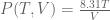
Now we can go further and say that both $T$ and $V$ are functions of time, $t$ . So we have:

$P(T(t),V(t))=\frac{8.31T(t)}{V(t)}=8.31T(t)[V(t)]^{-1}$ .

Read the rest of this entry »

MA1008: Exercise 3.3 Q.4 (ii)

February 7, 2011 in MA 1008 | Leave a comment

Express every solution of the given system as the sum of a specific solution plus a solution of the associated homogeneous system:

$2x_1+x_2-x_3-x_4=-1$

$3x_1+x_2+x_3-2x_4=-2$

$-x_1-x_2+2x_3+x_4=2$

$-2x_1-x_2+2x_4=3$

Solution: This question essentially asks you to use Theorem 3.4. Theorem 3.4 states that to solve the linear system of equations;

$A\mathbf{X}=\mathbf{b}$ (*)

it is sufficient to find some/ any (among all the solutions – if one exists) solution $\mathbf{X}_1$ , find the solution to the homogeneous system, $\mathbf{X}_0$ :

$A\mathbf{X}=\mathbf{0}$ ,

and that the general solution to (*) will be $\mathbf{X}_1+\mathbf{X_0}$ .

Realistically you wouldn’t use this method to solve this problem (Q.4 (ii)) – we are more seeing how this theorem works as ye will be using it later in solving linear differential equations.

Read the rest of this entry »

MA 1008: Integration by Partial Fractions Question

January 11, 2011 in MA 1008 | Leave a comment

This question was asked at Monday’s tutorial (10/01/11) but the fire alarm went off mid-solution

Section 6.4, Q. 5

Evaluate the following integral:

$\int\frac{(x-1)\,dx}{x^3-x^2-2x}$

Solution

(Remarks in italics are by me and would not be required in an exam situation)

Simplify the integrand to get it into a usable form:

$I=\int\frac{(x-1)\,dx}{x(x^2-x-2)}=\int\frac{(x-1)\,dx}{x(x-2)(x+1)}$

Rule 1 (Section 6.4)

Given a rational function $P(x)/Q(x)$ with $\text{deg}(P)<\text{deg}(Q)$ , such that $Q(x)$ factors into non-repeated linear terms:

$Q(x)=(a_1x+b_1)(a_2x+b_2)\cdots(a_nx+b_n)$

(non-repeated means that no linear term is equal to a constant multiple of another; e.g. $(a_ix+b_i)=k(a_jx+b_j)$ for $i\neq j$ , $k\in \mathbb{C}$ )

Then

$\frac{P(x)}{Q(x)}=\frac{A_1}{a_1x+b_1}+\frac{A_2}{a_2x+b_2}+\cdots+\frac{A_n}{a_nx+b_n}$

for some constants $A_1,A_2,\dots,A_n\in\mathbb{C}$ .

Read the rest of this entry »

MA 1008: Taylor Series Question

December 13, 2010 in MA 1008 | Leave a comment

Section 8.8, Q. 4

Find the Taylor series expansion of the function $\ln (1+x)$ about the point $x=1$ .

(This question was asked at Friday’ tutorial but, with one eye on the answer given, I was unable to do it. Having looked at the problem again I’m sure that the question should have been:)

Find the Taylor series expansion of the function $\ln x$ about the point $x=1$ .

(I have indicated this issue to Prof. Stynes)

Solution

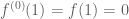
The Taylor series of any infinitely differentiable function about a point $x=a$ is given by the power series:

$f(x)\approx \sum_{n=0}^\infty \frac{f^{(n)}(a)}{n!}(x-a)^n$

Computing the first few derivatives of $f(x)=\ln x$ :

$\left.f^{(0)}(x)=\ln x\right|_{x=1}=0$

$\left.f'(x)=x^{-1}\right|_{x=1}=1$

$\left.f''(x)=(-1)x^{-2}\right|_{x=1}=-1$

$\left.f'''(x)=(-1)(-2)x^{-3}\right|_{x=1}=2$

$\left.f^{(iv)}(x)=(-1)(-2)(-3)x^{-4}\right|_{x=1}=-6$

$\vdots$

$\left.f^{(n)}(x)=(-1)^{n+1}(n-1)!x^{-n}\right|_{x=1}=(-1)^{n+1}(n-1)!$

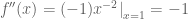
This is valid for $n\geq 1$ . At $n=0$ , $f^{(0)}(1)=f(1)=0$ . Hence we have;

$f(x)\approx \sum_{n=1}^\infty \frac{(-1)^{n+1}(n-1)!}{n!}(x-1)^n$

$f(x)\approx \sum_{n=1}^\infty \frac{(-1)^{n+1}}{n}(x-1)^n$ $\Box$

Leaving Cert: Integration

November 22, 2010 in General, Grinds, Leaving Cert, MA 1008 | Leave a comment

A short note covering integration for Leaving Cert maths.

(Please note that the proof of the Fundamental Theorem of Calculus inside isn’t quite correct. We need the Mean Value Theorem to prove it but the one in here is just for illustrative purposes.)

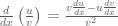
The Quotient Rule for Differentiation

November 3, 2010 in Grinds, Leaving Cert, MA 1008, MS 2001 | 5 comments

Here we present the proof of the following theorem:

Let $f,g:\mathbb{R}\rightarrow\mathbb{R}$ be functions that are differentiable at some $a\in\mathbb{R}$ . If $g(a)\neq 0$ , then $f/g$ is differentiable at $a$ with

$\left(\frac{f}{g}\right)'(a)=\frac{f'(a)g(a)-f(a)g'(a)}{[g(a)]^2}$

Quotient Rule

Remark: In the Leibniz notation,

$\frac{d}{dx}\left(\frac{u}{v}\right)=\frac{v\frac{du}{dx}-u\frac{dv}{dx}}{v^2}$

Proof: Let $q=f/g$ :

$q(a+h)-q(a)=\frac{f(a+h)}{g(a+h)}-\frac{f(a)}{g(a)}$

$=\frac{f(a+h)g(a)-f(a)g(a+h)}{g(a+h)g(a)}$

$=\frac{f(a+h)g(a)\overbrace{-f(a)g(a)+f(a)g(a)}^{=0}-f(a)g(a+h)}{g(a+h)g(a)}$

$=\frac{g(a)[f(a+h)-f(a)]-f(a)[g(a+h)-g(a)]}{g(a+h)g(a)}$

$\Rightarrow \frac{q(a+h)-q(a)}{h}=\frac{g(a)\left[\frac{f(a+h)-f(a)}{h}\right]-f(a)\left[\frac{g(a+h)-g(a)}{h}\right]}{g(a+h)g(a)}$

Letting $h\rightarrow 0$ on both sides:

$q'(a)=\left(\frac{f}{g}\right)'(a)=\frac{g(a)f'(a)-f(a)g'(a)}{[g(a)]^2}$ $\bullet$

Making sense of Algebra

October 26, 2010 in Grinds, Leaving Cert, MA 1008, MS 2001 | Leave a comment

Hopefully. The following note (in progress) might help you understand the power and proper functioning of basic real algebra Short_note_on_algebra

	J.P. McCarthy on MATH6040: Spring 2022, Week…
	J.P. McCarthy on MATH6040: Spring 2022, Week…
	J.P. McCarthy on MATH7019: Winter 2020, Week…
	J.P. McCarthy on MATH7019: Winter 2020, Week…
	A Sufficient Conditi… on Almost All Trees have Quantum…

Category Archive

A Strategy for AntiDifferentiation

Project Maths: A More Geometric Approach to De Moivre’s Theorem and Complex Roots

Introduction

Complex Numbers

Definition

MA 1008: Summer 2010, Q. 9 (b)

MA1008: Exercise 4.13

The Question

Solution

MA1008: Exercise 3.3 Q.4 (ii)

MA 1008: Integration by Partial Fractions Question

MA 1008: Taylor Series Question

Leaving Cert: Integration

The Quotient Rule for Differentiation

Making sense of Algebra

Recent Comments

Categories

J.P. McCarthy Maths

Category Archive

Share this:

Like this:

Introduction

Complex Numbers

Definition

Share this:

Like this:

Share this:

Like this:

The Question

Solution

Share this:

Like this:

Share this:

Like this:

Share this:

Like this:

Share this:

Like this:

Share this:

Like this:

Share this:

Like this:

Share this:

Like this:

Recent Comments

Categories