EDIT: two years later, I considered instead this at the level of the Tannaka–Krein categories. If at parameter , then if and only if . This may still be true, but I tried to relax to and this doesn’t work for , the half-liberated orthogonal group. For every , because in , quotienting to forces the isotropy to be commutative. This is related to “uniformity” in the sense of Banica.
The following is an approach to the maximality conjecture for which asks what happens to a counterexample when you quotient . If is noncommutative, you generate another counterexample .}
Most of my attempts at using this approach were doomed to fail as I explain below.
Let be a quantum permutation group with (universal) algebra of continuous functions generated by a fundamental magic representation . Say that is classical when is commutative and genuinely quantum when is noncommutative.
Definition 1 (Commutator and Isotropy Ideals)
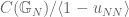
Given , the commutator ideal is given by:
The isotropy ideal is given by:
Lemma 1
The commutator ideal is equal to the ideal
Proof:
with a similar statement for .
On the other hand:
Proposition 1
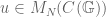
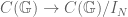
The commutator and isotropy ideals are Hopf*-ideals. The quotient gives a classical permutation group , the classical version, and the quotient giving an isotropy quantum subgroup. If is classical, this quotient is the isotropy subgroup of for the action .
Via , the classical permutation group is a quantum subgroup . It is conjectured that for all it is a maximal subgroup.
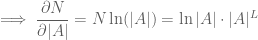
This is just a little exercise in partial differentiation
Introduction
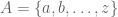
So, you have a password of length from an alphabet . Suppose you have a choice to increase the length, , vs the alphabet size . Which will make your password more secure?
In this sense we will assume that passwords are subject only to random guesses, and so we make the simple assumption that given the data , the larger the number of possible passwords, the more secure the password.
The set of passwords is . This has size .
Simple Numerics
A simple approach is to simply make a table:
An eyeballing of this will tell you that most of time it appears that increasing the length is preferable to increasing the alphabet size. But then again, alphabet size jumps tend to be larger, e.g. 26 to 52, 52 to 62, etc.
Suppose you have a length password from the alphabet . Are you better off going to length , or going to the alphabet of size , with the capital letters and the numebers? As it happens, it depends on . For , you should increase the length, but for , you should double the size of the alphabet. This is typical.
Some analysis
Consider a password from a set of . Consider the two options, for constant :
increase the alphabet size: , or
increase the password length .
If we look what these do to the number of passwords:
vs
,
we are comparing to , and are constant, we are comparing the exponential function and the polynomial function . While increasing the password length initially can do better, as and particularly increases, the exponential function speeds past the polynomial function, so eventually, it will make more sense to increase the alphabet size. Our eyeballing has let us down.
For example, from the table above, at and , it doesn’t appear to be even close, here at , and , you get far more security increasing the length.
But for a fixed , there exists a length for which it makes more sense to increase the alphabet by a factor of . The answer is 61.
So, if you have a length 61 password from an alphabet of size 20, you are better off increasing the alphabet size.
I guess what is relevant here are the following questions: at (adding the special characters), what are the answers?
If , and , you could increase the length of the password rather than jumping to .
If , and , you could increase the length of the password rather than jumping to .
If , and , you could increase the length of the password rather than jumping to .
Going to special characters only makes sense in our framework if there is also a password length condition of 10 or more.
Partial Differentiation
This wasn’t even what I wanted to do here, which was to approximate this question using partial differentiation. In all these questions we are asking about what happens to when we change and keep constant and vice versa. So partial differentiation. I guess the problem is and are discrete, rather than continuous, but sure and are perfectly good functions to differentiate. Let .
Even I can differentiate with respect to (in fact, on first go I wrote with respect to here, and got it wrong!):
.
We might use some logs to differentiate with respect to :
.
These partial derivatives estimate that if (a change of and ,
,
so, approximately, we are left comparing and . And here we see vs … eventually if both grow, giving us the same answer as before.
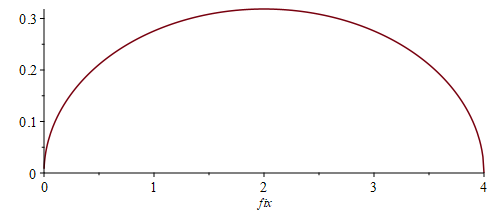
Consider the symmetric group . Let count the number of fixed points of a permutation . Where , we have that for a random permutation chosen with respect to the uniform distribution, the converges in distribution to in the sense that:
.
In this note we will look at the distribution in the case where the uniform distribution is conditioned on .
Theorem
Let be chosen according to the distribution uniform on permutations for which one is a fixed point. The number of fixed points has distribution in the sense that, where ,
.
Proof: What can be shown, ostensibly from stuff from the quantum permutation side of the house is that, where is integration against the uniform distribution, and is integration against the uniform distribution on permutations with one a fixed point, that, for :
,
the -st Bell number. Now consider the moments of :
,
using the fact that the Bell numbers are the moments of that Poisson distribution and the standard recurrence for the Bell numbers.
Local vs Global Conditioning of Quantum Permutations
In the quantum case we define
,
where is the fundamental magic representation. The moments of with respect to the Haar state are the Catalan numbers and it follows that the law of is a Marchenko-Pastur distribution, with density
:
Note that when we measure the Haar state with some finite spectrum version of we find:
the probability of finding an integer number of fixed points is zero, and
independently of , the probability of finding more than four fixed points is zero.
In the classical case above when we chose the permutation uniformly from those who fix one, there are two ways of viewing it:
we pick an element of that fixes one, OR
we consider the isotropy subgroup and choose our permutation from .
Classically, these are the same thing. In the quantum case these two things can be interpreted differently. The second case is quite clear in the quantum case. For , we take the isotropy via the quotient .
The analogue of the uniform distribution on here is the Haar idempotent . Note this maps to . Now, using the fact that , the Catalan number, we have that the moments of with respect to is the binomial transform of the Catalan numbers (the binomial transform of is ). It follows, using similar stuff to the above, that the distribution of with respect to is just a shifted version of Marchenko–Pastur:
I guess this is marginally more interesting than the unshifted version.
Now, what about an analogue of “we pick an element of that fixes one”. So if we take the Haar state and measure the observable that asks of a quantum permutation, does it fix one, we get, conditioned on this, the state:
.
And, it turns out, as above, using stuff from the quantum permutation side of the house:
.
Quite quickly from here we find that the density of the distribution of with respect to is
This is so interesting:
it doesn’t change the support — we still find between 0 and 4 fixed points,
we have a new symmetry about , we had another unexpected symmetry here.
the mean jumps from one to two, that is not unexpected, but
the mode jumps from zero to two!
even though we have observed one to one, there can still be less than one fixed point when we measure… and this happens with probability .
The next obvious question is what happens with:
Epilogue?
So what about this local vs global conditioning? Well, no matter what subsequent measurements are made to , we will always find that one is a fixed point. That conditioning is ‘global’.
This is not the case with , and why the support of the law is not bounded above one, like that of the globally conditioned . In fact, there is a non-zero probability that is observed to fix two but then subsequently not fix one anymore. That conditioning was only local: the probability that fixes one is 100%… but subsequent measurements can destroy that conditioning… it is only local.
We finished our work on Laplace’s Equation and then started – and finished looking at the Heat Equation.
Students who missed the lecture on Wednesday can catch up with the Lecture videos on Canvas.
We looked at Lab 7, based on Laplace’s Equation
Here on is provisional on when I go on paternity leave
Week 10
We will have tutorial time towards the 40% Written Assessment on Tuesday and Wednesday.
For Lab 8, the theory is examinable in the final written assessment but the VBA not examinable outside of Autumn repeat exam.
If I go on paternity leave a number of videos will have been produced:
an intro to Lab 8,
and outro to Lab 8,
four hours and 10 minutes of worked examples
You will be instructed to replace your four hours of lab and lecture time with engagement with these materials.
Week 11
I will almost certainly be on paternity leave. Your VBA 2 assessment will take place and it will be invigilated. NOTE DME2D will have their assessment at A285 and NOT B151 (at the usual time slot)
You will be instructed to replace your two hours of lecture time with engagement with the four hours and 10 minutes of worked examples.
Week 12
I will probably be on paternity leave. Your Written Assessment 2 will take place in the Melbourne.
You will be instructed to replace your Tuesday lecture time with engagement with the four hours and 10 minutes of worked examples.
If I am back from paternity leave your Tuesday lecture will be a tutorial.
Study
Study should consist of
doing exercises from the notes
completing VBA exercises
Student Resources
Please see the Student Resources tab on the top of this page for information on the Academic Learning Centre, etc..
Students who did not take advantage of the ample tutorial time this week (and those who did) are free to email me questions over Easter. Please send screenshots of your attempts.
15% Assignment 2
Assignment 2 is in the manual. It could be started now.
Week 9
We had a bumper week of Chapter 3 tutorials.
Week 10
I will probably not be on paternity leave yet, in which case we will have a final Chapter 3 tutorial on Tuesday before doing systems of differential equations on Wednesday and Thursday, with some tutorial time possible on Thursday.
If I do go on paternity leave, a colleague of mine is due to take ye. If it happens that this cover is late, only coming on Thursday, I will have pre-recorded lectures on systems of differential equations which you should watch instead of the lectures on Tuesday and Wednesday. Then my colleague will do a Chapter 3/ systems of differential equations tutorial with you on Thursday.
Week 11
I will be on paternity leave.
Tuesday will be a tutorial on systems of differential equations and then ye will work on double integration and when we finish that section we will have tutorials.
Week 12
I might be back from paternity leave.
Tuesday will be a tutorial on double integration and then ye will work on triple integration. When finished ye will have tutorial time on that topic.
Week 13, Review Week
We will have tutorial time.
Study
Please feel free to ask me questions about the exercises via email or on this webpage.
Student Resources
Please see the Student Resources tab on the top of this page for information on the Academic Learning Centre, etc..
Again, things are more serious now as we start Chapter 3. We must work hard on this material:
because without doing so you could be very, very lost on 15% Assignment 2 (and 35% exam question), and
because if you are going into Level 8 Structural Engineering it will be assumed that you are competent with the Chapter 3 material
Students who missed today, Thursday 14 March should really watch the videos covering Section 3.4 before Tuesday.
Week 8
The week will be focused on finishing the part of Chapter 3 examinable in Assignment. We did this, by looking at partial fractions, the inverse Laplace transform, and the application of the Laplace Transform to differential equations. We managed some tutorial time on Wednesday but the double was all lecture.
15% Assignment 2
Assignment 2 is in the manual, has a hand-in date of 12 April, and once you have had some tutorial time, you can start this.
Week 9
This will be a bumper week of Chapter 3 tutorials.
Week 10
I will probably not be on paternity leave yet, in which case we will have a final Chapter 3 tutorial on Tuesday before doing systems of differential equations on Wednesday and Thursday, with some tutorial time possible on Thursday.
If I do go on paternity leave, a colleague of mine is due to take ye. If it happens that this cover is late, only coming on Thursday, I will have pre-recorded lectures on systems of differential equations which you should watch instead of the lectures on Tuesday and Wednesday. Then my colleague will do a Chapter 3/ systems of differential equations tutorial with you on Thursday.
Week 11
I will be on paternity leave.
Tuesday will be a tutorial on systems of differential equations and then ye will work on double integration and when we finish that section we will have tutorials.
Week 12
I might be back from paternity leave.
Tuesday will be a tutorial on double integration and then ye will work on triple integration. When finished ye will have tutorial time on that topic.
Week 13, Review Week
We will have tutorial time.
Study
Please feel free to ask me questions about the exercises via email or on this webpage.
Student Resources
Please see the Student Resources tab on the top of this page for information on the Academic Learning Centre, etc..
The VBA results have been released and all groups will have one chance to get some quick feedback on what they submitted. If this doesn’t or hasn’t worked for you, please feel free to send an email.
I have set a target of Week 9 for your Written Assessment results.
Week 8
We continued with Chapter 2, describing the implementation of the Gauss-Seidel method. We have stopped (geddit) short of giving the stopping rule, ye will see this on Tuesday.
We did Lab 6 on boundary value problems, and it is relevant for VBA Assessment 2 in Week 11.
Week 9
We will finish our work on Laplace’s Equation and then start looking at the Heat Equation.
We will look at Lab 7, based on Laplace’s Equation
Because every lab counts, the Bank Holiday labs of DME2A are going to be rescheduled to Tuesday: on Tuesday March 19 we will have the following:
DME2A, 14:40-16:20, DME2E 16:20-18:00, A285
Here on is provisional on when I go on paternity leave
Week 10
We will finish our work on the Heat Equation and have tutorial time on Wednesday.
For Lab 8, the theory is examinable in the final written assessment but the VBA not examinable outside of Autumn repeat exam.
If I go on paternity leave a number of videos will have been produced:
a video covering the last lecture of new material,
an intro to Lab 8,
and outro to Lab 8
two hours and 40 minutes of worked examples
You will be instructed to replace your four hours of lab and lecture time with engagement with these materials.
Week 11
I will almost certainly be on paternity leave. Your VBA 2 assessment will take place and it will be invigilated.
You will be instructed to replace your two hours of lecture time with engagement with the two hours and 40 minutes of worked examples.
Week 12
I will probably be on paternity leave. Your Written Assessment 2 will take place in the Melbourne.
You will be instructed to replace your Tuesday lecture time with engagement with the two hours and 40 minutes of worked examples.
If I am back from paternity leave your Tuesday lecture will be a tutorial.
Assessment
See Canvas for the assessment schedule.
Study
Study should consist of
doing exercises from the notes
completing VBA exercises
Student Resources
Please see the Student Resources tab on the top of this page for information on the Academic Learning Centre, etc..
Again, things are more serious now as we start Chapter 3. We must work hard on this material:
because without doing so you could be very, very lost on 15% Assignment 2 (and 35% exam question), and
because if you are going into Level 8 Structural Engineering it will be assumed that you are competent with the Chapter 3 material
Timetable Change
The Monday class is now moved to A243L at 13:00 on Tuesdays. This allows us to spread out tutorial time better, and hopefully is logistically better for you.
Week 7
On Monday, we had a final Chapter 2 tutorial.
Then the rest of the class will be given over to partial fractions and then the inverse Laplace transform.
On Wednesday and Thursday we had some tutorial time on partial fractions and the cover up method.
Week 8
The week will be focused on finishing Chapter 3.
15% Assignment 2
Assignment 2 does not yet have a hand-in date (watch this space). Assignment 2 is in the manual, and once you finish the exercises in the manual you will be in a great position to start.
Week 9
This should be a bumper week of Chapter 3 tutorials if we have finished Chapter 3.
The below is very much provisional
Week 10
We will do systems of differential equations.
Week 11
We will work on double integration and when we finish that section we will have tutorials.
Week 12
We will work on triple integration. When finished we will have tutorial time on that topic.
Week 13, Review Week
We will go through an exam paper, answer questions, and have tutorial time as appropriate.
Study
Please feel free to ask me questions about the exercises via email or on this webpage.
Student Resources
Please see the Student Resources tab on the top of this page for information on the Academic Learning Centre, etc..
In VBA we finished what we are doing on Lab 4 and then looked at Lab 5. Lab 5 is not examinable as VBA but the theory of it, the theory of RK, that is examinable in Written Assessments 1 and 2. Some students instead used the time to prepare for Written Assessment 1.
Assessment Corrections
Let us set a target of Week 8 for your VBA results and Week 9 for your Written Assessment results.
Week 8
We will continue with Chapter 2.
Lab 6 is on boundary value problems and relevant for VBA Assessment 2 in Week 11.
Week 9
Section 2.1
Lab 7
Because every lab counts, the Bank Holiday labs of DME2A are going to be rescheduled to Tuesday: on Tuesday March 19 we will have the following:
DME2A, 14:40-16:20, DME2E 16:20-18:00, A285
Here on is provisional:
Week 10
Section 2.2
Lab 8 (theory examinable in final written assessment but VBA not examinable outside of Autumn repeat exam)
Week 11
Finish Section 2.2 and then tutorial time
Assessment
See Canvas for the assessment schedule.
Study
Study should consist of
doing exercises from the notes
completing VBA exercises
Student Resources
Please see the Student Resources tab on the top of this page for information on the Academic Learning Centre, etc..


![\displaystyle J_N=\langle [u_{ij},u_{kl}]\,\mid\, 1\leq i,j,k,l\leq N\rangle.](https://s0.wp.com/latex.php?latex=%5Cdisplaystyle+J_N%3D%5Clangle+%5Bu_%7Bij%7D%2Cu_%7Bkl%7D%5D%5C%2C%5Cmid%5C%2C+1%5Cleq+i%2Cj%2Ck%2Cl%5Cleq+N%5Crangle.&bg=ffffff&fg=545454&s=0&c=20201002)


![\begin{aligned} [u_{i_2j_2},u_{i_3j_1}] & =u_{i_2j_2}u_{i_3j_1}-u_{i_3j_1}u_{i_2j_2} \\ \implies u_{i_1j_1}[u_{i_2j_2},u_{i_3j_1}] & = u_{i_1j_1}u_{i_2j_2}u_{i_3j_1}\qquad (i_1\neq i_3)\\ \implies u_{i_1j_1}u_{i_2j_2}u_{i_3j_1} & \in J_N, \end{aligned}](https://s0.wp.com/latex.php?latex=%5Cbegin%7Baligned%7D+%5Bu_%7Bi_2j_2%7D%2Cu_%7Bi_3j_1%7D%5D+%26+%3Du_%7Bi_2j_2%7Du_%7Bi_3j_1%7D-u_%7Bi_3j_1%7Du_%7Bi_2j_2%7D+%5C%5C+%5Cimplies+u_%7Bi_1j_1%7D%5Bu_%7Bi_2j_2%7D%2Cu_%7Bi_3j_1%7D%5D+%26+%3D+u_%7Bi_1j_1%7Du_%7Bi_2j_2%7Du_%7Bi_3j_1%7D%5Cqquad+%28i_1%5Cneq+i_3%29%5C%5C+%5Cimplies+u_%7Bi_1j_1%7Du_%7Bi_2j_2%7Du_%7Bi_3j_1%7D+%26+%5Cin+J_N%2C+%5Cend%7Baligned%7D&bg=ffffff&fg=545454&s=0&c=20201002)
![\begin{aligned} [u_{i_1j_1},u_{i_2j_2}] & =u_{i_1j_1}u_{i_2j_2}-u_{i_2j_2}u_{i_1j_1} \\ & =u_{i_1j_1}u_{i_2j_2}\sum_{k=1}^Nu_{i_1k}-\sum_{l=1}^{N}u_{i_1l}u_{i_2j_2}u_{i_1j_1} \\ & = u_{i_1j_1}u_{i_2j_2}u_{i_1j_1}+u_{i_1j_1}u_{i_2j_2}\sum_{k\neq j_1}u_{i_1j_1}u_{i_2j_2}u_{i_1k}-\\&u_{i_1j_1}u_{i_2j_2}u_{i_1j_1}\sum_{l\neq j_1}u_{i_1l}u_{i_2j_2}u_{i_1j_1}\\ \implies [u_{i_1j_1},u_{i_2j_2}]& \in K_N \end{aligned}](https://s0.wp.com/latex.php?latex=%5Cbegin%7Baligned%7D+%5Bu_%7Bi_1j_1%7D%2Cu_%7Bi_2j_2%7D%5D+%26+%3Du_%7Bi_1j_1%7Du_%7Bi_2j_2%7D-u_%7Bi_2j_2%7Du_%7Bi_1j_1%7D+%5C%5C+%26+%3Du_%7Bi_1j_1%7Du_%7Bi_2j_2%7D%5Csum_%7Bk%3D1%7D%5ENu_%7Bi_1k%7D-%5Csum_%7Bl%3D1%7D%5E%7BN%7Du_%7Bi_1l%7Du_%7Bi_2j_2%7Du_%7Bi_1j_1%7D+%5C%5C+%26+%3D+u_%7Bi_1j_1%7Du_%7Bi_2j_2%7Du_%7Bi_1j_1%7D%2Bu_%7Bi_1j_1%7Du_%7Bi_2j_2%7D%5Csum_%7Bk%5Cneq+j_1%7Du_%7Bi_1j_1%7Du_%7Bi_2j_2%7Du_%7Bi_1k%7D-%5C%5C%26u_%7Bi_1j_1%7Du_%7Bi_2j_2%7Du_%7Bi_1j_1%7D%5Csum_%7Bl%5Cneq+j_1%7Du_%7Bi_1l%7Du_%7Bi_2j_2%7Du_%7Bi_1j_1%7D%5C%5C+%5Cimplies+%5Bu_%7Bi_1j_1%7D%2Cu_%7Bi_2j_2%7D%5D%26+%5Cin+K_N+%5Cend%7Baligned%7D&bg=ffffff&fg=545454&s=0&c=20201002)


 from an alphabet
  . Suppose you have a choice to increase the length,
  , vs the alphabet size
  . Which will make your password more secure?
 , the larger the number of possible passwords, the more secure the password.
 . This has size
  .
. 
 . Are you better off going to length
  , with the capital letters and the numebers? As it happens, it depends on
  , you should increase the length, but for
  , you should double the size of the alphabet. This is typical.
 :
:  , or
, or .
. vs
vs ,
, to
to  , and
, and  are constant, we are comparing the exponential function
  and the polynomial function
  . While increasing the password length initially can do better, as
  and particularly
  and
and  , it doesn’t appear to be even close, here at
  , and
, and  , you get far more security increasing the length.
 . The answer is 61.
 (adding the special characters), what are the answers?
 , and
, and  .
. , you could increase the length of the password rather than jumping to
  .
. , you could increase the length of the password rather than jumping to
  .
. and
and  are perfectly good functions to differentiate. Let
  .
. .
. 

 .
. and
and 
 ,
, and
and  . And here we see
  vs
vs  if both grow, giving us the same answer as before.
 . Let
. Let  count the number of fixed points of a permutation
  . Where
 ![X\sim \mathrm{Poi}[1]](https://s0.wp.com/latex.php?latex=X%5Csim+%5Cmathrm%7BPoi%7D%5B1%5D&bg=ffffff&fg=545454&s=0&c=20201002) , we have that for a random permutation
, we have that for a random permutation  chosen with respect to the uniform distribution, the
  converges in distribution to
  in the sense that:
![\displaystyle \lim_{N\to \infty}\mathbb{P}[\mathrm{fix}_N(\xi_N)=m]=\mathbb{P}[X=m]](https://s0.wp.com/latex.php?latex=%5Cdisplaystyle+%5Clim_%7BN%5Cto+%5Cinfty%7D%5Cmathbb%7BP%7D%5B%5Cmathrm%7Bfix%7D_N%28%5Cxi_N%29%3Dm%5D%3D%5Cmathbb%7BP%7D%5BX%3Dm%5D&bg=ffffff&fg=545454&s=0&c=20201002) .
. .
. ![1+\mathrm{Poi}[1]](https://s0.wp.com/latex.php?latex=1%2B%5Cmathrm%7BPoi%7D%5B1%5D&bg=ffffff&fg=545454&s=0&c=20201002) in the sense that, where
in the sense that, where ![\displaystyle \lim_{N\to \infty}\mathbb{P}[\mathrm{fix}_N(\xi_N)=m]=\mathbb{P}[X=m-1]](https://s0.wp.com/latex.php?latex=%5Cdisplaystyle+%5Clim_%7BN%5Cto+%5Cinfty%7D%5Cmathbb%7BP%7D%5B%5Cmathrm%7Bfix%7D_N%28%5Cxi_N%29%3Dm%5D%3D%5Cmathbb%7BP%7D%5BX%3Dm-1%5D&bg=ffffff&fg=545454&s=0&c=20201002) .
. is integration against the uniform distribution, and
  is integration against the uniform distribution on permutations with one a fixed point, that, for
  :
: ,
, -st Bell number. Now consider the moments of
  :
:![\displaystyle \sum_{t=0}^\infty t^k\mathbb{P}[1+X=t]=\sum_{t=0}^\infty t^k\mathbb{P}[X=t-1]](https://s0.wp.com/latex.php?latex=%5Cdisplaystyle+%5Csum_%7Bt%3D0%7D%5E%5Cinfty+t%5Ek%5Cmathbb%7BP%7D%5B1%2BX%3Dt%5D%3D%5Csum_%7Bt%3D0%7D%5E%5Cinfty+t%5Ek%5Cmathbb%7BP%7D%5BX%3Dt-1%5D&bg=ffffff&fg=545454&s=0&c=20201002)


 ,
, ,
, is the fundamental magic representation. The moments of
  :
:
 and choose our permutation from
  .
. , we take the isotropy
  via the quotient
  .
. . Note this maps
  . Now, using the fact that
  , the
, the  is
is  ). It follows, using similar stuff to the above, that the distribution of
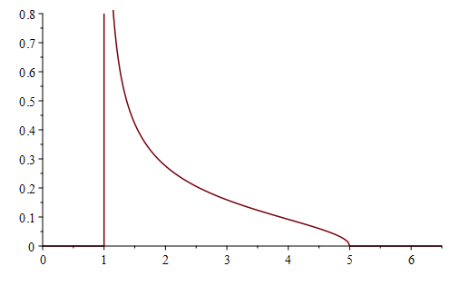
 that asks of a quantum permutation, does it fix one, we get, conditioned on this, the state:
 .
. .
. is
is 
 , we had another unexpected symmetry
  .
.

Recent Comments