
I am emailing a link of this to everyone on the class list every week. If you are not receiving these emails or want to have them sent to another email address feel free to email me at jippo@campus.ie and I will add you to the mailing list.
Week 2
In week 2 we began to look at homogenous second order linear differential equations (with constant coefficients). These are differential equations of the form
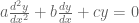
where 


Fact 1
In general, if the roots of of this equation are 


where 

The real constants are to be determined by two boundary/initial conditions of the form 

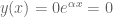
There were possible complications however. If the roots are real and equal, say both

which at the end of the day is just ‘constant’ 
A good question at this point is how do we know there are more solutions (as we are going to say below)? Before we even answer this we should note that the 


We can do even better and design an actual damped harmonic oscillator/door closer such that the roots of the auxiliary equation are repeated. Now open the door to a width of 1 m and release from rest: 
If we do go deeper into the mathematics we can go away and prove that the solution space of the linear operator:
is two dimensional (briefly, needs two independent components) so there must be another solution. As it turns out, and we did the calculation in class, 
Fact 2
If the roots of the auxiliary equation to (*) are repeated, then the general solution is given by

A second complication that can occur is if the roots are complex. The Conjugate Root Theorem says that the roots of the auxiliary equation will be of the form

whenever the coefficients

for some possibly complex constants
However it can be shown that this solution can be rewritten. This yields another fact:
Fact 3
If the roots of the auxiliary equation to (*) are complex, then the general solution is given by

for real constants 

Week 3
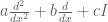
In week 3 we asked what happens when the right hand side of (*) is not zero but rather some non-zero function of 

This is then a non-homogeneous second order linear differential equation. We were able to prove the following fact:
N-HSOLDE Fact
The general solution of (**) is given by
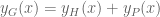
where 

The trick is to find a particular solution based on what 
If 


If 


Tutorials
Tutorials Tuesday 6 – 8 pm start this week. If you have any questions this will be the time to ask. After that we will have tutorials in weeks 4, 5, 6, 8, 10, 12.
Test 1
As it stands the test will be on in week 6 although I might be moving this to week 7. I will have a sample test for ye very soon.
Notes
The notes on second order linear differential equations that I handed out. Note that you should be attempting the exercises.

Leave a comment
Comments feed for this article