Taken from Franz & Gohm.
Let return to the map  considered in the beginning of the previous section. If
  is a group, then is called a left action of on
  , if it satisfies the following axioms expressing associativity and unit (
 ),
),
 , and
, and 
for all  ,
,  ; and where
  is the identity. As before we have the unital *-homomorphisms
  . Actually, in order to get a representation of on
  , i.e.
  for all
  we modify the definition and use
  . (Otherwise we get an anti-representation. But this is a minor point at this stage). In the associated coaction
  the axioms above are turned into the coassociativity and counit properties. These make perfect sense not only for groups but also for quantum groups and we state them at once in this more general setting. We are rewarded with a particular interesting class of quantum Markov chains associated to quantum groups which we call random walks and are the subject of this lecture.
A bialgebra is a unital associative algebra  equipped with two unital algebra homomorphisms
  and
and  such that

 .
.
To see where these are motivated from (i.e. quantising  ), we will examine these relations for, once again,
  . The naive view at this point would suggest that the comultiplication and counit are of the form:
 ,
,
 .
.
In fact this is the correct form of the comultiplication. Now for the first condition above:
 .
.
Having done a few calculations, I think that this equals:
 .
.
Similarly,
 .
.
I’m sure this is supposed to encode the associativity law  , but I can’t really see how exactly. In fact seeing where the ‘group encodings’ are coming from exactly is the biggest problem. I can see how they’re supposed to encode associativity, the identity and inverses but Thomas Cooney defines
  by
by  and I’m failing to get to these relations via this definition.
Next the condition on the counit. First the calculations:
 .
.
Similarly,  . It is a little easier to see the encoding here of
  .
.
If has an involution  such that
  and
and  are *-homomorphisms, then we call a *-bialgebra.
Let  and suppose
  . If there exists furthermore a linear map
  (called the antipode) satisfying
 ,
,
then we call a *-Hopf algebra. If we define a multiplication map  ,
,  , then this can be rewritten as

Definition A.1
A finite quantum group is a finite dimensional C*-Hopf algebra.
Note that finite dimensional C*-algebras are very concrete objects, namely they are multi-matrix algebras  (see Theorem 6.3.8). Not every multi-matrix algebra carries a Hopf algebra structure. The simplest example is that of the group algebra of a finite group. For example, the direct sum must contain a one-dimensional summand to make possible the existence of a counit.
Proof : The only homomorphisms from  occur for
  (Second Example)
Let be a finite quantum group with comultiplication and counit . A C*-algebra  is an -comodule algebra if there exists a unital *-algebra homomorphism
  such that
 ,
, .
.
Such a map  is a coaction.
To see that this is the ‘encoding’ of an action we examine this for the algebra of a finite group. The coaction is going to be related to the action of on itself — morryah the coaction of onto  (?). Let
  . The calculations show, for
  :
:
 .
.
 .
.
This is supposed to encode the fact, that for actions, ,
,
but once again I can’t see it exactly.
Now for the other condition:
 .
.
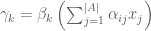
This we might be able to do something with. has basis  , we can write, for complex numbers
  :
:


 .
.
Well this means that if  , then the ‘
 ‘ coaction of acts on by the vector
  — in other words it does nothing really, consolidating .
If we start with such a coaction then we can look at the quatum Markov chain constructed in the previous section in a different way. Define for  :
:
 ,
,

where  is inserted at the
  -th copy of . We can interpret the
  as non-commutative random variables. Note that the are identically distributed (Cf. the construction of a random walk on a finite group [Equation 1.5, page 15]). Further the sequence
  is a sequence of tensor independent random variables (their ranges commute and the state acts as a product state on them). The convolution
  is another random variable, defined by
 .
.
where  . By my calculations, this is just
  ?!! This would give the homomorphism property though.
In a similar way we can form the convolution of the among each other. By induction we can prove the following formulas for the random variables  of the chain.
Proposition 3.1


 .
.
Proof: That the second formula is true is quickly shown using a telescoping argument. Let  be the proposition that the third formula is true. Clearly
  and
and  is true. Assume that
  is true:
 .
.
What about  ? Again using :

 ,
,
where the  term is in the
  st position
Note that by the properties of coactions and comultiplications the convolution is associative and we do not need to insert brackets. The statement  can be put into words by saying that the Markov chain associated to a coaction is a chain with (tensor-) independent and stationary increments (???). Using the convolution of states we can write the distribution of
  as
as  . For all
  and the Transition operator satisfies
 ,
,
and thus from this we can verify that
 .
.
Proof of the first equality: First off a few calculations of powers of the transition operator:


Inductively,

Now hitting this with  we hit the
  term. We must get an expression for
  therefore. We have that
  ,
,  . Now
. Now


 .
.
Hence, inductively:
 .
.
Hitting this with  yields
  we have that
i.e. given , the semigroup of transition operators  and the semigroup
  of convolution powers of the transition state are essentially the same thing.
A quantum Markov chain associated to such a coaction is called a random walk on the -comodule algebra . We have seem that in the commutative case this construction describes the action of a group on a set and the random walk derived from it. Because of this background, some authors call a coaction the action of a quantum group.
Theorem A.2
Let be a finite quantum group. Then there exists a unique state  on such that
 , for all .
The state is called the Haar State of . The defining property (above) is called left-invariance. On finite (and more generally on compact) quantum groups, left invariance is equivalent to right invariance; i.e. the Haar state satisfies also
 .
.
One can show that it is a faithful trace, i.e.  implies
  and
and
 , for
, for  .
.
Using the unique Haar state, we also get the distinguished inner product on , namely for :
 .
.
This theorem is stated in the paper without proof. A proof is found here (including the faithfulness property). This is the approach we follow.
Proof : Let be a finite quantum group and let  be it’s dual. We know that the functionals on ,
  are of the form:
 ,
,
for and  .
.
Claim 1
There exists a non-zero element  such that
  .
.
Proof : Let  be a basis for and let
  be the dual basis (of ). Suppose that
  and let
  for
for  . For any
  define by:
 .
.
Take (this first line makes no sense to me actually: I thought the counit was a homomorphism so that  . I therefore cannot see how the counit gets inside the bracket to take advantage of the
  relation?? Therefore I might just ‘take his word’ as I can’t follow an argument I don’t understand.)
This proves the existence of left Haar functional on . By duality we also get the existence of a left Haar measure on (I presume this means via the map  ,
,  ??).
??).
Uniqueness will follow easily from the next result.
Claim 2
Let  be a non-zero element of such that for all
  . Then the map
  ,
,  is bijective.
Proof : It is enough to prove that this map is injective. We can show that the map is surjective if for any complex numbers  ,
,  (where
  ),
),  we can solve the
  equations for the
  unknowns
  :
:
where  …(!)
…(!)
So assume  and
and  (the map is linear so one-to-one at zero implies injective)… actually I’m totally confused looking at this so I’m just going to assume the existence of the Haar measure at this point
Concerning stationarity we get:
Proposition 3.2
For a state on the following assertions are equivalent:

 for all states
  on
on  , where is the Haar state on .
Proof : That (a)

(b) can be seen by applying
ti both sides of (a).
I’m not so sure of how to go the other way although it is probably pretty clear. (b) (c) is patently obvious.
Assuming (c) and using the invariance properties of
we get for all states
on
:
 … I can’t make head nor tail of this!
 The Eight-Dimensional Kac-Paljutkin Quantum Group
In this section we give the defining relations and the main structure of an eight-dimensional quantum group introduced by Kac and Paljutkin. This is actually the smallest finite quantum groups that is not a group algebra (e.g.  ). In other words, it is the non-commutative C*-Hopf algebra of smallest dimension (Franz & Gohm talk about both the group algebra and the algebra of functions on the group: what is the difference? He also talks about commutative and cocommutative. What is the difference?).
Consider the multi-matrix algebra  , with the usual multiplication and involution. We shall use the basis
  (with
(with  defined in the same way) and
 ,
,
with the other  defined in the same way. The algebra is an eight-dimensional C*-algebra. Its unit is of course
  . We shall need the trace
  on .
on .
 .
.
Note that Tr is normalised to be equal to one on minimal projections ( ).
).
The following defines a coproduct on ,

 ,
,

 ,
,

 ,
,

 ,
,

 ,
,

 ,
,

 ,
,

 .
.
The counit is given by (looking at this we can see the relationship between the counit and the comultiplication with respect to the unit and multiplication in a commutative, group algebra, case. To encode  any time there is a term of the form
  , there must be a term of the form
  — to capture the left and right symmetry
  . This also shows that, in this case,
  must contain and to encode
  ):
):
 .
.
The antipode is the transpose map, i.e.
 , and
, and  .
.
Which I’ve checked satisfies  for
for  and
and  .
.
The Haar State
Finite quantum groups have unique Haar elements satisfying  ,
,  and
and
 , for all .
For the Kac-Paljutkin quantum group, it is easy to see that  . An invariant functional is given by
  with
with  and
and  . On an arbitrary element of the action of is given by
 .
.
Normalising so that  , we get the Haar state
  .
.
The dual of
The dual of a finite quantum group is again a finite quantum group. Its morphisms are the duals of the morphisms (do these look right???) of , e.g.
 ,
, 
and
 ,
,  .
.
The involution of is given by  for
for  , (this is done by showing that the routine calculation
  holds for all
  ).
).
To show that is indeed a C*-algebra, once can show that the dual regular action of on defined by  for , , is a faithful *-representation of with respect to the inner product on defined by

for .
For the Kac-Paljutkin quantum group the dual actually turns out to be isomorphic to itself.
Denote by  the basis of that is dual to
  , i.e. the functionals on defined by
 ,
,  ,
,
 ,
,  ,
,
for  ,
,  ,
,
We leave the following as an exercise (yeah; what is a minimal projection? I have a little proposition (16.5 (a)) but I can’t quite seem to make sense of how it applies to ):
The functionals
 ,
,
 ,
,
 ,
,
 ,
,
are minimal projections in , Furthermore
 ,
,
 ,
,
 ,
,
 ,
,
are matrix units; i.e. satisfy the relations
 and
and  ,
,
and the mixed products vanish,
 ,
,  ,
,  .
.
Therefore  as an algebra. But actually,
  and
and  even defines a C*-Hopf algebra isomorphism from to .
The States on 
On  there exists only one state, the identity map. States on
  are given by density matrices, i.e. positive semi-definite matrices with trace one. More precisely, for any state
  on there exists a unique density matrix
  such that
 ,
,
for all  . The
. The  density matrices can be parameterised by the unit ball
  ,
,
 .
.
A state on is a convex combination of states on the four copies of and a state on . All states on can therefore be parameterised by  and the set
 .
.
Example 3.3
Consider the commutative subalgebra  of the Kac-Paljutkin Quantum Group with standard basis
  and component-wise multiplication. Franz & Gohh on page 9 define an -coaction which makes into an -comodule algebra.
Let be an arbitrary state on . It can be parameterised by the  and
and  . Then the transition operator
  on
on  has a matrix representation, with respect to the basis
  , given on p.10 of Franz & Gohm.
The state  defined by
  for
for  is invariant, i.e. we have

for any state on .


1 comment
Comments feed for this article
September 21, 2011 at 4:58 pm
An alternative quantisation of a Markov chain? or Why do we need Coalgebras? « J.P. McCarthy: Math Page
[…] category theory. At times I can see that the coalgebra is encoding a lot (see some remarks here and here), but really I haven’t a clue what’s going […]