Taken from Hopf Algebras by Abe. This is not even nearly finished however I pressed publish instead of save draft… oh well.
In this section, we give the definition of Hopf algebras and present some examples. We begin by defining coalgebras, which are in a dual relationship with algebras., then bialgebras and Hopf algebras as algebraic systems in which the structures of algebras and coalgebras are interrelated by certain laws.
1.1 Coalgebras
We define a coalgebra dually to an algebra. Given an algebra  and algebra homomorphisms
  and
and  , we call
  or just a coalgebra when we have:
 ,
,
(the coassociative law).
 ,
,
(the counitary property)
The maps  and
and  are called the comultiplication map and the counit map of , and together they are said to be the structure maps of the coalgebra .
Now suppose we are given two coalgebras  and
and  . A linear map
  satisfying the conditions
 ,
, 
is called a coalgebra morphism.
For algebras and  we define a linear map
 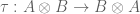 by
by  for
for  ,
,  . If a coalgebra satisfies
 ,
,
then is said to be cocommutative. If and are two coalgebras, the tensor product  becomes a coalgebra with structure maps
 ,
,
 ,
,
which we call the tensor product of and . If  are cocommutative, then is a direct product of cocommutative coalgebras where the canonical projections
 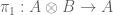 ,
,  are respectively given by
  and
and  for
for  ,
,  .
.
When a subalgebra  of a coalgebra satisfies the condition
  , then
  becomes a coalgebra with the restrictions of
  to as the structure maps. Such a is called a subcoalgebra of .
For algebras and , if we define a map  by
by
 ,
,
where  ,
,  , and , then
  is an injective linear map (Suppose that
  . That is to say that for all
  ,
,
 .
.
and by the no divisors theorem  or
or  for all , . Hence
  or
or  and
and  .). Given a coalgebra , let
  denote the dual of .
 ,
,
 ,
,
 becomes an algebra, which we call the dual algebra of .
I’m not sure exactly what  and
and  are here. I’m supposing that they are the adjoints of the linear maps and but I haven’t ever gone through the construction via the inducement of a map
  from a linear map
  — which is an approach mentioned here. The only natural inducement I can think of is follows. Let
  be a linear map between vector spaces
  and
and  . Now define a linear map
  by
by  .
.
Now let  be a bilinear form. A bilinear form induces linear maps
  and
and 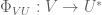 :
:
,  where
where 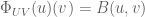 ,
,
and similarly for  .
.
If and are inner product spaces, I can also define a bilinear maps  using the inner product of and
  :
:
 .
.
By fixing  , I could define a linear functional on and hence we have a map
  given by:
 .
.
I’m happy enough here to invoke Riesz representation theorem and the existence of  such that
 ,
,
where I define  in the obvious way. So what I have is , but I really want to identify
  with a
  and this will hopefully tell me what and are. Let
  and define , by
 .
.
I think this is the identification I need. For example, take  . In this construction,
  so that
 ,
,
where  is the inner product adjoint of . Similarly
  .
.
In general, is not necessarily an isomorphism. Thus we cannot define a coalgebra structure on the dual space of an algebra in a similar fashion. However, if is a finite dimensional vector space, then  turns out to be a vector space isomorphism; if
  ,
,  are the structure maps of , then by setting
  ,
,  , we see that
  becomes a coalgebra.
Firstly, I can’t see how  can be a comultiplication for . We require
  , yet
, yet  doesn’t act on — it acts on
  . I’m going to try
  — at least
  . Let and
  . We know that
 .
.
We might want to show that  so that
  is the inverse of when we restrict to
  . This is equivalent to
  or
or  and even further
  . From here we may be able to identify elements of with elements of
  uniquely and hopefully pull the coassociativity of from this via
  . I don’t know if this is necessarily true but I can still look at statements about and turn them into statements about — which has coassociativity. If we note that
  , then
  so we need to show that
 , for all .
Could we express  in terms of alone? We start by noting that
  by
by
 .
.
While this is indeed progress and I’m getting better at visualising what’s going on I’ll leave it there for now…
This is called the dual coalgebra of .
Example 2.1 (Modified)
Let be a vector space with an orthonormal basis  . Define linear maps:
 ,
, 
for  by
by  ,
,  , then
  becomes a coalgebra (
 ). The dual space
  can be identified with
  where the dual algebra structure of is given by
 ,
,
 ,
,
for  , and
, and  .
.
First let us examine  . Take an element
  . Now
. Now  and
and  . So if I can show that
  we are done as this will yield
  . Now, for all
  we have
 ,
,
 ,
,
 .
.
Now 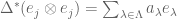 and from this it is clear that
 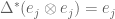 so we are done.
Now looking at the map  . Now let
  so that we want
 .
.
The only way this makes any kind of sense is if  , where
  is the constant function on
  .
.
Example 2.2
Let be a vector space with a countable orthonormal basis  and define
 ,
,  .
.
to obtain the coalgebra (). We will briefly look at the structure of the dual algebra of . If we let  be defined by
 ,
,  .
.
then can be written
 , where
  .
.
With regard to multiplication on , we have

 .
.
Thus the relation  holds, and we get
  for
for  . Therefore we see that is isomorphic to the ring
 ![\mathbb{C}[x_1]](https://s0.wp.com/latex.php?latex=%5Cmathbb%7BC%7D%5Bx_1%5D&bg=ffffff&fg=545454&s=0&c=20201002) .
.
Example 2.3
Let  be a natural number and set
  and the vector space with basis . Defining
 ,
,  ,
,
we obtain a coalgebra (). The dual space of is a vector space of dimension  and if we define
  by
by
 ,
,
then  is a basis for . By identifying
  with the
  square matrix
 ![[a_{ij}]_{ij}](https://s0.wp.com/latex.php?latex=%5Ba_%7Bij%7D%5D_%7Bij%7D&bg=ffffff&fg=545454&s=0&c=20201002) , becomes the algebra
, becomes the algebra  of all square matrices with complex entries.
Notation for Coalgebra Operations
In general, the notation used for operations of coalgebras is not as concise as that for operations of algebras. The following notation is effective in simplifying various types of operations. Given a colalgebra and , we can write
 , for
, for  .
.
We write this formally as
 ,
,
and for linear operators (or functionals)  , we write
 .
.
Moreover, since the associative law holds, we have
 ,
,
and in general we define  , and
, and
 ,
,
for  , and write
 .
.
Using this method of notation, the counitary property may be expressed as
 .
.
Exercise 2.1
Prove the following equalities
 ,
,
 ,
,
 .
.
Solution : First write
 .
.
Now we note that, using the counitary property, we can write
 .
.
But

 .
.
Now use the counitary and coassociativity to write
 .
.
This yields:
 .
.
After we make the identifications  , this is the first set of equalities.
By applying coassociativity we have
 .
.
A quick calculation shows the first of the second set of equalities. A calculation shows that
 .
.
By coassociativity:
 .
.
Now hit  with this:


by the first of the equality above.
For the third equality, the right-hand side is given by:
 .
.
Now by using coassociativity and the counitary propery twice:

 .
.
So all three sets of inequalities are proven.
Theorem 2.1.1
Given a vector space  , suppose that there are linear maps
 ,
,  ,
,  ,
, 
such that  is an algebra and
  is a coalgebra. Then the following are equivalent.
- and are coalgebra morphisms.
- and are algebra morphisms.
 ,
,  ,
,  ,
,  .
.
Proof : The conditions under which is an algebra morphism are (see here):
(a) 
(b) 
The conditions under which is an algebra morphism are
(c) 
(d)  .
.
On the other hand, is a coalgebra morphism exactly when it satisfies conditions (a) and (c) (); and is a coalgebra morphism if it satisfies conditions (b) and (d) (). This fact allows us to conclude that 1.  2.
2.
Now assume (2). The equation

implies that .
The equation  we get that
  .
.
The equation  yields .
Finally the equation  yields
  . Clearly (iii)
  (ii) and we are done
When a vector space together with linear maps  satisfies one of the equivalent conditions of Theorem 2.1.1, then
  , or simply , is called a bialgebra. Given two bialgebras and
  , when a linear map
  is an algebra morphism and is also a coalgebra morphism, then
  is called a bilalgebra morphism.
If a subspace of a bialgebra is a subalgebra as well as a subcoalgebra, then becomes a bialgebra, and is called a sub-bialgebra of . Moreover, if a bialgebra is finite dimensional, then a bialgebra structure may be defined on its dual  , which we call the dual bialgebra of .
Example 2.4
Let  be a semigroup with identity, and let
  be the free complex vector space generated by . In the sense of example 2.1, has a coalgebra structure when we consider as a basis for . With regard to these two structures, admits a bialgebra structure. Such a bialgebra is called a semigroup bialgebra. In particular, when is a group, it is called a group bialgebra. The dual space
  can be identified with
  , and in particular, when is finite, then becomes a dual bialgebra of . The algebra structure of is the one described in Example 1.5, and its coalgebra structure is given for
  ,
,  , and the identity element
  by
by
 ,
,  .
.
I’m not one hundred percent what these  are — do they just mean:
 and
and  .
.
When an element of a coalgebra is such that  and
and  , then is said to be a group-like element. We denote the set of all group-like elements by
  .
.
Theorem 2.1.2
Let be a coalgebra.
(i) The elements of are linearly independent. Thus  may be regarded as a subcoalgebra of .
(ii) When is a bialgebra,  is a semigroup with respect to multiplication, and the subspace of generated by is a sub-bialgebra of isomorphic to the semigroup bialgebra
  of .
of .
Proof : Suppose that the elements in are linearly dependent, and let  be the least value for a set of elements of to be linearly dependent. Then there exist
  such that
  are linearly independent and
  can be written
 ,
,  and
and  .
.
Since
 , and also
 .
.
Hence we may write
 .
.
Since  is a set of linearly independent elements of
  (), this implies that all of the
  or
or  — and also that the mixed terms
  all vanish. Hence
  and
and  , which contradicts the choice of (i.e.
  is a set of
  linearly dependent elements. We also have no problem when
  ). Hence the elements of are linearly independent. It is apparent that is a subcoalgebra of .
To prove part (ii), the first thing is to show that  . Note that associativity is clear as
  . Using the equation
 ,
,
we can show that  for all
  , as required
An element  of a bialgebra (resp a coalgebra which has only one group-like element, i.e.
  ) which satisfies
  (resp.
  ) is called a primitive element. The set of all primitive elements of is denoted by
  . Now we have the following.
Theorem 2.1.3
If is a bialgebra, then  is a subspace of , and for
  , we have
 ![[x,y]=xy-yx\in P(H)](https://s0.wp.com/latex.php?latex=%5Bx%2Cy%5D%3Dxy-yx%5Cin+P%28H%29&bg=ffffff&fg=545454&s=0&c=20201002) . Thus has the structure of a Lie Algebra. Moreover, if
. Thus has the structure of a Lie Algebra. Moreover, if  ,
,  .
.
Proof : If , then
![\Delta([x,y])=\Delta x\Delta y-\Delta y\Delta x](https://s0.wp.com/latex.php?latex=%5CDelta%28%5Bx%2Cy%5D%29%3D%5CDelta+x%5CDelta+y-%5CDelta+y%5CDelta+x&bg=ffffff&fg=545454&s=0&c=20201002)


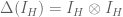
![=[x,y]\otimes 1+1\otimes [x,y]](https://s0.wp.com/latex.php?latex=%3D%5Bx%2Cy%5D%5Cotimes+1%2B1%5Cotimes+%5Bx%2Cy%5D&bg=ffffff&fg=545454&s=0&c=20201002) .
.
Thus ![[x,y]\in P(H)](https://s0.wp.com/latex.php?latex=%5Bx%2Cy%5D%5Cin+P%28H%29&bg=ffffff&fg=545454&s=0&c=20201002) . For we have
. For we have
 .
.
Hence
Example 2.6
Let  , and let
  be the coalgebra defined in Example 2.2. Defining a multiplication by
 ,
,
becomes an algebra. With respect to these two structures, becomes a bialgebra. By setting
 ,
,
we obtain  , which implies
  for . Thus as an algebra, is isomorphic to the polynomial ring
 ![\mathbb{C}[d_1]](https://s0.wp.com/latex.php?latex=%5Cmathbb%7BC%7D%5Bd_1%5D&bg=ffffff&fg=545454&s=0&c=20201002) in one variable. In this situation,
in one variable. In this situation,  .
.
1.2 Hopf Algebras
Given a coalgebra  and an algebra . If
  ,
,

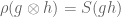
is said to be the convolution of  and . If
  , then
  , which is simply the definition of the product of two functions on
  via multiplication on .
  becomes an algebra with structure maps
 ,
,  .
.
Given a bialgebra , let  and
and  respectively denote regarded simply as an algebra and a coalgebra, and view
  as an algebra via convolution as defined above. When the identity map
  of is an invertible element of with respect to multiplication on , the inverse of
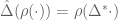
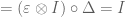
  is called the antipode of . The antipode is the element which satisfies one of the following equivalent conditions


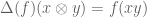
A bialgebra with antipode is called a Hopf algebra. Let  be Hopf algebras and let
  be the antipodes of respectively. When a bialgebra morphism satisfies the condition
 ,
,
is called a Hopf algebra morphism.
Example 2.7
Denote by  the group bialgebra of a group
  (see Example 2.4). We define a linear map
  by
by  for
for  . Then
 , .
, .
Thus is the antipode of , so that becomes a Hopf algebra. is an anti-automorphism of as an algebra and  is the identity map of .
Theorem 2.1.4
The following properties hold for an antipode of a Hopf algebra .
 , for all
  .
. ; namely
  .
. .
.
 ; in other words.
- The following conditions are equivalent
6.
If is commutative or cocommutative, then  .
.Remark
1. and 2. imply that is an anti-algebra morphism; 3. and 4. imply that
is an anti-coalgebra morphism.
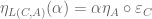
Proof : 1. Define elements of  in the following manner. For , we write
 ,
,  ,
,  .
.
Now, if we show that  , then we get
  , which would prove 1.
I can show that
 , and
, and
 ,
,
but can’t see how this implies that — which is the technique Abe uses. To show  is just a calculation.
2. Since  ,
,  , we have
 .
.
3. From the fact that  and…
and…

implies
.
.
.

Leave a comment
Comments feed for this article