Taken from Random Walks on Finite Quantum Groups by Franz & Gohm
In this section we will show how one can recover a classical Markov chain from a quantum Markov chain. We will apply a folklore theorem that says one gets a classical Markov process, if a quantum Markov process can be restricted to a commutative algebra.
We might like to do more. This result recovers a Markov chain — if the quantum process is in fact a random walk on a finite quantum group can we recover the group, the transition probabilities (yes), the driving probability measure??
Conjecture
If we restrict a random walk on a finite quantum group to a commutative subalgebra we can recover a random walk on a finite group.
For random walks on quantum groups we have the following result.
Theorem 6.1
Let  be a finite quantum group
  a random walk on a finite dimensional -comodule algebra
  , and
, and  a unital abelian sub-*-algebra of . The algebra is isomorphic to the algebra of functions on a finite set, say
  where
where  .
.
If the transition operator  of leaves invariant, then there exists a classical Markov chain
  with values in
  , whose probabilities can be computed as time-ordered moments of , i.e.

for all  and
and  .
.
Proof : We use the indicator functions  ,
,
 ,
,  ,
,
as a basis for  . They are positive, therefore
 , …,
, …, 
are non-negative. Since furthermore
 ,
,
these numbers define a probability measure on .
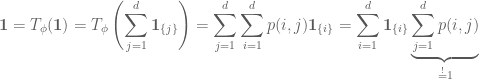
Define now  by
by
 .
.
Since  is positive (
 ), we have
  for . Furthermore,
  implies
 .
.
Hence ![[p(i,j)]_{1\leq i,\,j\leq d}](https://s0.wp.com/latex.php?latex=%5Bp%28i%2Cj%29%5D_%7B1%5Cleq+i%2C%5C%2Cj%5Cleq+d%7D&bg=ffffff&fg=545454&s=0&c=20201002) is a stochastic operator.
is a stochastic operator.
Therefore there exists a unique Markov chain with initial distribution  and transition matrix
  .
.
We show by induction that the equation in the theorem statement holds.
For  this is clear by the definition of
  . Suppose now that
  and . Then we have


Remark
If the condition that leaves  invariant is dropped, then one can still compute the “probabilities” but in general they are no longer positive or even real, and so it is impossible to construct a classical stochastic process from them.
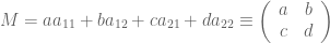
Example
The comodule algebra  that we considered here is abelian, so we can take
  . For any pair of states
  on and
  on (the Kac-Paljutkin quantun group), we get a random walk on and a corresponding Markov chain on
  . We identify
  with by
  for
for  .
.
The initial distribution is given by  and the transition matrix is given by (3.1) on page 10.
Example
Let us now consider random walks on the Kac-Paljutkin quantum group itself. For the defining relations, the calculation of the dual of and a parameterisation of all states see here. Let us consider here transition states of the form
 ,
,
with the  positive real numbers summing to
  .
.
The transition operators  of these states leave the abelian subalgebra
  invariant. The transition matrix of the associated classical Markov chain on
  that arises by identifying
  for has the form
 .
.
This actually the transition matrix of a random walk on the the group  .
.
A pertinent point here is that in this case we actually have a random walk on a finite group rather than just an ordinary Markov chain. If we had an ordinary Markov chain there is no distinction between and  . In fact a quick calculation shows that this is the stochastic operator of the random walk driven by the probability
 ,
,  ,
,  and
and  .
.
Could it be the the stochastic operator of a random walk on — well not always because these have to be circulant matrices. The only time when this stochastic operator is circulant is when  .
.
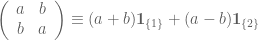
The subalgebra  is also invariant under these states, acts on it by

for
 ,
,  ,
,
with
 ,
,  ,
,  .
.
Let  be a unit vector in
  and denote by
  , the orthogonal projection onto
  . The maximum abelian subalgebra
  is in general not invariant under .
For example, for  we get the algebra
 .
.
It can be identified with  via
via
 .
.
Specialising to the transition state  and starting from the Haar measure
  , we see that the time-ordered joint moment is negative and thus can not be obtained from a classical Markov chain.
Example
For states in  , the centre
  of is invariant under . A state on parameterised by (B.1) belongs to this set if and only if
  (). With respect to the basis
  of
of  we get
![{T_\phi}_{|Z(A)}=\left(\begin{array}{ccccc}\mu_1&\mu_2&\mu_3&\mu_4&\mu_5\\\mu_2&\mu_1&\mu_4&\mu_3&\mu_5\\\mu_3&\mu_4&\mu_1&\mu_2&\mu_5\\\mu_4&\mu_3&\mu2&\mu_1&\mu_5\\[1ex] \mu_5/4&\mu_5/4&\mu_5/4&\mu_5/4&1-\mu_5\end{array}\right)](https://s0.wp.com/latex.php?latex=%7BT_%5Cphi%7D_%7B%7CZ%28A%29%7D%3D%5Cleft%28%5Cbegin%7Barray%7D%7Bccccc%7D%5Cmu_1%26%5Cmu_2%26%5Cmu_3%26%5Cmu_4%26%5Cmu_5%5C%5C%5Cmu_2%26%5Cmu_1%26%5Cmu_4%26%5Cmu_3%26%5Cmu_5%5C%5C%5Cmu_3%26%5Cmu_4%26%5Cmu_1%26%5Cmu_2%26%5Cmu_5%5C%5C%5Cmu_4%26%5Cmu_3%26%5Cmu2%26%5Cmu_1%26%5Cmu_5%5C%5C%5B1ex%5D+%5Cmu_5%2F4%26%5Cmu_5%2F4%26%5Cmu_5%2F4%26%5Cmu_5%2F4%261-%5Cmu_5%5Cend%7Barray%7D%5Cright%29&bg=ffffff&fg=545454&s=0&c=20201002) .
.
This is not the stochastic operator of a random walk on a finite group — it is not doubly stochastic. Furthermore this puts paid to the conjecture made above (however I am under the impression that there is an isomorphism between abelian finite quantum groups and finite groups — more on this later).
For Lévy processes or random walks on quantum groups there exists another way to prove the existence of a classical version that does not use the Markov property. We will illustrate this with an example.
Example
We consider restrictions to the centre of . If  , then
  and therefore
![[a\otimes 1_A,\Delta (b)]=0](https://s0.wp.com/latex.php?latex=%5Ba%5Cotimes+1_A%2C%5CDelta+%28b%29%5D%3D0&bg=ffffff&fg=545454&s=0&c=20201002) for all
for all  .
.
This implies that the range of the restriction  of any random walk on to is commutative, i.e.
![[j_\ell(a),j_n(b)]](https://s0.wp.com/latex.php?latex=%5Bj_%5Cell%28a%29%2Cj_n%28b%29%5D&bg=ffffff&fg=545454&s=0&c=20201002)
![=[(j_0\star k_1\star\cdots \star k_\ell)(a),(j_0\star k_1\cdots \star k_n(b))]](https://s0.wp.com/latex.php?latex=%3D%5B%28j_0%5Cstar+k_1%5Cstar%5Ccdots+%5Cstar+k_%5Cell%29%28a%29%2C%28j_0%5Cstar+k_1%5Ccdots+%5Cstar+k_n%28b%29%29%5D&bg=ffffff&fg=545454&s=0&c=20201002)
![=[(j_0\star k_1\star\cdots\star k_\ell)(a),(j_0\star k_1\star\cdots\star k_\ell)(b_{(1)})(k_{\ell+1}\star\cdots\star k_n)(b_{(2)})]](https://s0.wp.com/latex.php?latex=%3D%5B%28j_0%5Cstar+k_1%5Cstar%5Ccdots%5Cstar+k_%5Cell%29%28a%29%2C%28j_0%5Cstar+k_1%5Cstar%5Ccdots%5Cstar+k_%5Cell%29%28b_%7B%281%29%7D%29%28k_%7B%5Cell%2B1%7D%5Cstar%5Ccdots%5Cstar+k_n%29%28b_%7B%282%29%7D%29%5D&bg=ffffff&fg=545454&s=0&c=20201002)
![=\nabla(j_\ell\otimes(k_{\ell+1}\star\cdots\star k_n))([a\otimes 1_A,\Delta (b)])=0](https://s0.wp.com/latex.php?latex=%3D%5Cnabla%28j_%5Cell%5Cotimes%28k_%7B%5Cell%2B1%7D%5Cstar%5Ccdots%5Cstar+k_n%29%29%28%5Ba%5Cotimes+1_A%2C%5CDelta+%28b%29%5D%29%3D0&bg=ffffff&fg=545454&s=0&c=20201002)
for all  and (I must admit I’m not sure of the calculus of these calculations). Therefore the restriction corresponds to a classical process.
Let us now takes states for which does not leave the centre of the Kac-Paljutkin quantum group invariant; for example
 for
for ![z\in [-1,1]](https://s0.wp.com/latex.php?latex=z%5Cin+%5B-1%2C1%5D&bg=ffffff&fg=545454&s=0&c=20201002) .
.
In this particular case we have the invariant commutative subalgebra  which contains the centre . If we identify with
  via ,
via ,  and
and  , then the transition matrix is given at the bottom of page 21.
The classical process corresponding to the centre arises from this Markov chain by “gluing” the two states  and
and  into one. More precisely, if is a Markov chain that has the same time-ordered moments as restricted to , and if
  is the mapping defined by
  for
for  and
and  , then
  with
with  , for
, for  , has the same joint moments as restricted to the centre of . Note that is not a Markov process.


Leave a comment
Comments feed for this article