
Exam Layout
Answer four questions: each worth the same marks.
1. Multiple Topics Question
(a) Interpolation (b) Linear Algebra (c) Laplace Methods
2. Interpolation
Finite Difference Methods, Least Squares, Lagrangian Interpolation
3. Linear Algebra
Gaussian Elimination with and without partial pivoting, Cramer’s Rule, Jacobi’s Method, Gauss-Siedel Method
4. Laplace Methods
Three differential equations
5. Multiple Integration
line integrals, double integrals with applications including second moment of area, triple integrals.

7 comments
Comments feed for this article
December 14, 2012 at 11:43 am
Student 28
Just saw your email with the triple integral example (pg 142) and on the very last integral I was wondering should not be from 0 to 3 rather than 0 to 2?
Sorry for annoying you again but I wanted to check the answers to Q3(a) on the sample paper you gave us (2009/10). I’ve tried it out and the answers I have are (i) 264 (ii) 14 and (iii) 196. If you have answers for this question could you let me know if I’ve done it right.
December 14, 2012 at 12:07 pm
J.P. McCarthy
You are absolutely correct that — corrected.
Firstly what we have is
We will not have an integral presented to us in this form. Rather the so that the integral is
The first line integral, without a picture. The line segment from is a line which cuts the
  -axis at
  and has a slope of 2. Hence the curve may be parameterised by
  and
and 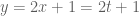 with
with  . Also
  and
and  . Hence we have
Your answer to the second integral is correct.
For the third integral, without a picture we have . Hence we can use the parameterisation
  and
and 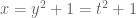 where
where  — morryah
  — runs from
  . We have
  and $dy=dt$. Hence our integral is
Regards and Happy Christmas,
J.P.
December 14, 2012 at 12:12 pm
Student 29
Can you take a look over my answer to
December 14, 2012 at 12:24 pm
J.P. McCarthy
The first problem in your solution is that you completely forgot about when you took the Laplace Transform.
After that things are good up until the point where correctly you infer that and
and  … which is O.K. except the same equation
also implies that (i.e. comparing the constant coefficients)… which is a bit of a problem.
Here I present a worked solution with (overly?) extensive explanations:
The first thing to do is the take the Laplace Transform of the differential equation. This transforms a differential equation with solution to an algebraic solution with solution
  — and algebraic equations are easier to solve.
Note that the Laplace Transform is linear, which means that we can transform term-by-term and pull out constants:
Now we have expressions for the Laplace Transform of the first and second derivatives in the tables. They are given in terms of the Laplace Transform of the solution, and the initial conditions (at time,
  ) of
) of  and
and  . The Laplace Transform of a constant is also in the tables:
  . Hence we have
Now we apply the initial/ boundary condition that :
:
Now we solve for :
:
We want to apply the inverse Laplace Transform to go from
  . Now the idea is that nothing like this is in the tables. We need to write this as a sum of simpler terms… partial fractions. The first thing to do is factorise the denominator
  inasmuch as possible. When you try and factor the quadratic it doesn’t seem to factor so we check
  . This means that the roots of the quadratic are complex. However the Factor Theorem says that
We have complex roots and hence cannot factor without complex numbers. Such a quadratic is not factorisable (such a quadratic is called irreducible over the real numbers).
O.K. we cannot factorise the denominator any further so what we must do now is associate to each term in the facorisation of the denominator a term in the partial fraction expansion. is a linear factor so begets a term of the form
Note that we may not use the cover-up method as we do not have a product of distinctive linear terms. Hence what we will do is write
write the partial fraction expansion as a single fraction again and compare.
Hence we want, for all values of ,
,
The denominators of these are the same so we need the numerators to be equal:
Note that these must be equal for all values of . Hence we could put
  and generate three equations in the three unknowns
  and hence find their values (note that the partial fraction expansion is unique — e.g. as opposed to fractions which can be expanded in different ways
  for example).
Alternatively we can do what you do which was multiply out and compare coefficients (this works because if for all
  then
then  ; e.g.
  after differentiating both sides with respect to
  ).
).
Hence we have ,
,  and — what we were missing —
  . Thence we have
  ,
,  and
and  . Thus we have
Now we know how to deal with . What about
  . All we can handle is, in terms of quadratics,
Hence all we can really say is that ‘kind of looks like’
  . Could we write
  in this form? Let’s try
Now this will be equal, again for all values of (cf. partial fraction expansion), if the coefficients are equal on both sides; i.e.
The first equation yields and hence the second reads
  . You can take
  . Hence we have
Now if we could write the second term here in the form
for some constants and
and  then we are well set. The first term here is a
  shifted sine, while the second is a
  shifted cosine. We have in the tables that
where . On the other hand we have that a
  shifted function is multiplied by
  by the inverse Laplace Transform:
To actually write
is not that easy and I don’t have a good way of doing it apart from playing around with the thing:
which is exactly the form we need. The first term is a shifted cosine while the second is a shifted sine. Now we send the whole thing back (note that the inverse Laplace Transform is also linear)
Sure enough (a good idea has a check to see is the initial condition satisfied) and also this function satisfies the differential equation.
Regards and Happy Christmas,
J.P.
December 14, 2012 at 1:42 pm
Student 30
Can you give a quick run through about the rules that are applied in the formula which I have outlined in green here. What are &
&  ?
?
December 14, 2012 at 1:45 pm
J.P. McCarthy
Suppose you get down to a point where your Laplace Transform looks like
where are constants but
  cannot be factorised any more because the roots are complex:
  .
.
All we can handle is, in terms of quadratics,
However all we can really say is that can be written as
  — once we complete the square. However if we could write
for some constants and
and  then we are well set. The first term here is a
  shifted sine, while the second is a
  shifted cosine. We have in the tables that
where . On the other hand we have that a
  shifted function is multiplied by
  by the inverse Laplace Transform:
To actually write
is not that easy and I don’t have a good way of doing it apart from playing around with the thing. The first term is a shifted cosine while the second is a shifted sine. Now we send the whole thing back (note that the inverse Laplace Transform is linear which means you can transform term-by-term and pull out constants):
There is an example of a question like this in the above comment.
Regards and Happy Christmas,
J.P.
December 14, 2012 at 3:02 pm
Nick
Ok thanks JP! Happy Christmas to you too! Thanks for all your help.
Nick