This is the first in a series of posts that are an attempt by me to understand why my Industrial Measurement and Control students need to study the Laplace Transform.

Consider a black box model that takes as an input signal a function x(t) and produces an output signal y(t). For reasons that are as of yet not clear to me, we can take all of the derivatives of y(t) (and x(t)) to vanish for t=0.

Definition

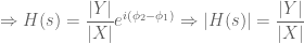
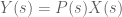
The transfer function of a black box model is defined as

\displaystyle H(s)=\frac{Y(s)}{X(s)},

where Y(s) and X(s) are the Laplace Transforms of y(t) and x(t).

Note we have the Laplace transform of a function f(t) is a function F(s) defined by

F(s)=\mathcal{L}\{f(t)\}=\int_{0}^\infty f(t)e^{-st}\,dt.

Poles of H(s) are complex numbers z such that X(z)=0. For example, for an input signal x(t)=e^t, the transfer function has a pole at s=1 as

\displaystyle F(s)=\frac{1}{s-1}.

If the coefficients of x(t) are real, then in general the poles of the transfer are real or come in conjugate root pairs.

Derivation of Formula for Transfer Function — Linear ODE Case

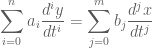
Consider a linear input/output system described by the differential equation:

\displaystyle \sum_{i=0}^na_i\frac{d^iy}{dt^i}=\sum_{j=0}^mb_j\frac{d^jx}{dt^j},

where we can take a_n=0.

If we assume that the input signal is of the form e^{st} then because the system is linear we must also have the output signal as y(t)=y_0e^{st}. Inserting these signals into the ODE yields:

\displaystyle y_0\sum_{i=0}^na_is^ie^{st}=\sum_{j=0}^mb_js^je^{st},

and so the response of the system can be described by the two polynomials
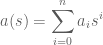
\displaystyle a(s)=\sum_{i=0}^na_is^i (with a_n=0)

and

\displaystyle b(s)=\sum_{j=0}^mb_js^j.

The polynomial a(s) is nothing but the characteristic/auxiliary equation of the associated homogenous system. If it is not everywhere zero then we have

\displaystyle y(t)=y_0e^{st}=\frac{b(s)}{a(s)}e^{st}=G(s)u(t).

Therefore, the transfer function is

\displaystyle H(s)=\frac{b(s)}{a(s)}=\frac{1/a(s)}{1/b(s)}.

Example: Complex Harmonic Signal

Suppose we have an input signal

\displaystyle x(t)=Xe^{i\omega t}=|X|e^{i\phi_1}e^{i\omega t},

and an output signal

\displaystyle y(t)=Ye^{i\omega t}=|Y|e^{i\phi_2}e^{i\omega t}.

Then we have

\displaystyle X(s)=\frac{|X|e^{i\phi_1}}{s-i\omega} and \displaystyle Y(s)=\frac{|Y|e^{i\phi_2}}{s-i\omega}

\displaystyle \Rightarrow H(s)=\frac{|Y|}{|X|}e^{i(\phi_2-\phi_1)}\Rightarrow |H(s)|=\frac{|Y|}{|X|}.

This |H(s)| is the gain. 

Example: Closed Loop Transfer Function

In this model, the output y(t) is measured and compared with the reference (ideal output) value r(t). The controller then takes the error, e(t)=\pm (y(t)-r(t)), and changes the input x(t) of the system under control, P, using some controller. This is known as a closed-loop controller or a feedback controller.

If we assume that the controller, system and sensor are linear and time-invariant (their transfer functions C(s), P(s) and F(s) do not depend on time), we can use the Laplace transform to analyse the system. We have

\displaystyle Y(s)=P(s)X(s),

\displaystyle X(s)=C(s)E(s) and

\displaystyle E(s)=R(s)-F(s)Y(s).

Some elementary algebra shows that
\displaystyle Y(s)=\left(\frac{P(s)C(s)}{1+F(s)P(s)C(s)}\right)R(s)=H(s)R(s).
If |P(s)C(s)|\gg1 and |F(s)|\approx 1 then we have that H(s)\approx 1 and so
Y(s)\approx R(s),
and so the output, y(t), tracks the reference value, r(t), quite well.
Advertisement