
Arguably, the three central concepts in the theory of differential calculus are that of a function, that of a tangent and that of a limit. Here we introduce functions and tangents.
Functions
When looking at differential calculus, two good ways to think about functions are via algebraic geometry and interdependent variables. Neither give the proper, abstract, definition of a function, but both give a nice way of thinking about them.
Algebraic Geometry Approach
Let us set up the plane, 

Now, perpendicular to the 
This is the plane,
Now points on the plane can be associated with a pair of numbers 

Similarly, I can take a pair of numbers, say (-1,3), and this corresponds to a point on the plane.
This gives a duality:
points on the plane 
Now consider the completely algebraic objects

These objects have as solutions pairs of numbers:


Now if we plot all the solutions of an equations we get a curve. When I say curve I just mean a set of points on the page.

Here we see the first four curves above plotted. The horizontal line is
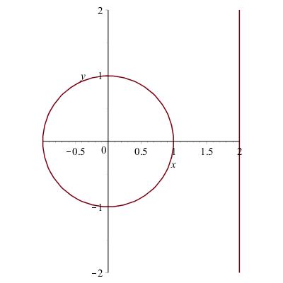
The solutions of the equation 
To play around with this go to Wolfram Alpha and input “plot some equation”. Some nice curves to plot may be found here.
This gives us another duality:
Points on a Curve (Geometry)
This means we can answer geometric questions using algebra and answer algebraic questions using geometry.
Algebraic Question to be Answered using Geometry
Let 


This set of simultaneous equations has __, __, __ or ___________ solutions.
Now there is a difference between the first four curves and the second two curves (above). For the first four curves, for each

Usually mathematicians are lazy so rather than writing stuff… we write

Such curves are the graphs of functions.
Therefore the circle and the vertical line 
The circle is, however, the graphs of two functions glued together:
Interdependent Variables Approach
Another way to think about functions is as a pair of variables 
To say that
These functions can be graphed by graphing all the points of the form:

where 

Example
The area, 
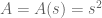
To plot this function we plot all pairs 


Tangents
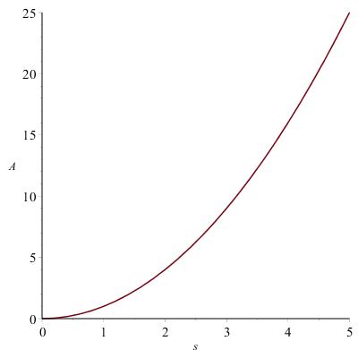
All of the functions above have one thing in common… when we zoom in on them they look like lines.
For example, consider the function 

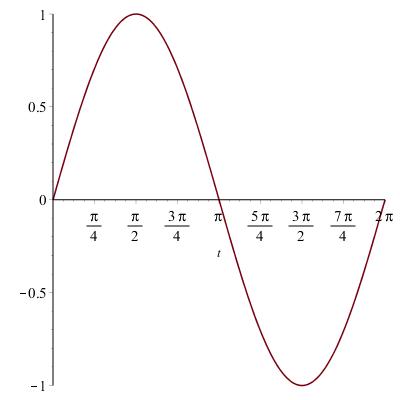
Take the point 

At the point 

The aim of calculus is to find the slope of these tangents. If we can find the slope of the tangent then we can write down the equation of the tangent.

2 comments
Comments feed for this article
December 15, 2016 at 3:26 pm
Tangents to Circles | J.P. McCarthy: Math Page
[…] I said in the previous post, there is a […]
June 5, 2018 at 4:48 pm
On Parallel and Perpendicular Lines | J.P. McCarthy: Math Page
[…] implies that the definitions are equivalent. This post introduces the idea of Duality: in this case between Geometry and Algebra. The power of this […]