
Distances between Probability Measures
Let 


The algebra 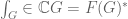
Define a (bijective) map 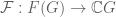

for 
Then, where 


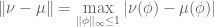
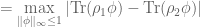
(Quantum Total Variation Distance (QTVD))
Standard non-commutative 

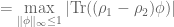
(supremum presentation)
In the classical case, using the test function 


In the classical case the set of indicator functions on the subsets of the group exhaust the set of projections in

(Projection Distance)
In all cases the quantum total variation distance and the supremum presentation are equal. In the classical case they are equal also to the projection distance. Therefore, in the classical case, we are free to define the total variation distance by the projection distance.
Quantum Projection Distance  Quantum Variation Distance?
Perhaps, however, on truly quantum finite groups the projection distance could differ from the QTVD. In particular, a pair of states on a 
The following are two solutions to this problem. The first used a bit of help on Math Stack Exchange, and the second a more elegant solution from Jean-Christophe Bourin (communicated by Uwe Franz). They are similar — the first constructing an explicit map, the second using a phase.
The Supremum is Attained at An Involution
Embed the multi-matrix 
Consider the supremum presentation. As everything is in finite dimensions, the supremum is actually a maximum. Suppose that the max is attained for a self-adjoint involutive 
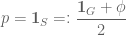
is a projection:
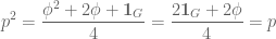
and 


If, however, there was a pair of states such that the max is not attained at an involution, then the projection distance for these two states would be strictly smaller than the QTVD.
Consider, therefore, two states on 

From here we use the argument of Hanno.
Define 

where 


Note that 


Now define the operator norm one diagonal matrix

Note

has trace equal to 


The Supremum is attained at a Phase
As above, define 


and so

Note now
but this upper bound is attained at
Conclusion
This means there is no counterexample to
Projection Distance = QTVD.
What this means is that we can take as a definition the quantum total variation distance to be the same as the classical total variation distance:

where 


2 comments
Comments feed for this article
November 16, 2017 at 9:12 pm
Random Walks on Quantum Groups: Outlook | J.P. McCarthy: Math Page
[…] It should also be possible to redefine the quantum total variation distance as a supremum over projections subsets via . If I can show that for a positive linear functional that then using these ideas I can. More on this soon hopefully. No, this approach won’t work. (I have since completed this objective with some help: see here). […]
February 16, 2018 at 5:40 pm
Random Walks: Questions for The Future | J.P. McCarthy: Math Page
[…] that the total variation distance is equal to the projection distance. Amaury has an a third proof. Amaury suggests that this should be true in more generality than the […]