
A Poker Hack
I told this story in class on Friday. I wasn’t sure if it was true but it appears that it is.
Texas Hold’Em Poker
‘Texas‘ is a poker game where a number of players sit around a table. Two cards are dealt to each player. There after follows a round of betting, the reveal of three more cards (the flop), more betting, another card (the turn), another round of betting, another card (the river), and another round of betting:

What we are interested in is what happens after all this, before another hand is dealt?
The deck is shuffled.
A shuffle is required to mix up the deck. Here we used three terms: deck, shuffle, mixed up. These can all be given a precise mathematical realisation (see the introduction here for more). Mixed up means ‘close to random’. Here let me introduce a mathematical realisation of random:
If one is handed a deck of cards, face down, and if each possible order of
the cards is equally possible then the deck is considered random.
Note there are 

One popular method of shuffling cards is the riffle shuffle. In a remarkable 1992 paper by Bayer & Diaconis, with a really cool name: Trailing the Dovetail Shuffle to Its Lair, it is shown that seven riffle shuffles are necessary and sufficient to get a deck close to random:

Here we see 


So the idea is after, say, ten shuffles (or, equivalently, about ten rounds of hands), the deck is mixed up or close to random: each of the 52! orders are approximately likely.
This says something quite remarkable about the uniqueness of card games. Imagine each of the approximately 8 billion people on Earth own a deck of cards. Suppose we all spent 8 hours a day for 50 years shuffling our cards… at one shuffle per minute that is only about 
This is a tiny, tiny, fraction of the 52! possible orders! Only approximately

of all decks have ever been seen… so the probability of two orders ever have been repeated is tiny. When you play a deck of cards, the likelihood is that no other deck of cards have ever been in that order!
Now when we move online we need an algorithm to shuffle the deck. One algorithm works as follows.
Number all the different orders from 

Start with a random number. This can be found by turning on a computer and having the computer record the number of milliseconds, 
The first deck used on the table is 
Now, from

using the recurrence:


Here 


using seed 
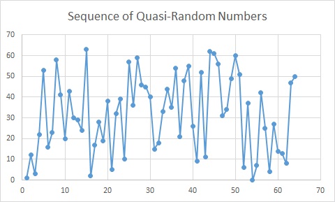
So an online poker site can start with a random deck, and using a quasi-random number generator recurrence, generate a list of random-looking decks.
However, a serious error was made by the those in charge of one particular site. The way they stored the deck orders was not enough to encode all possible orders and in fact (using 32 bits rather than the 200+ necessary) only a tiny, tiny proportion of all possible deck orders were stored.
This resulted in carnage: carnage that you can read more about here.
Exercises
- How many possible decks orders are there?
- What does it mean to say a deck of cards is random?
- Roughly, how many riffle shuffles are required to randomise a deck of cards?
- Briefly describe how to produce a quasi-random sequence using a linear recurrence.
Spin The Wheel
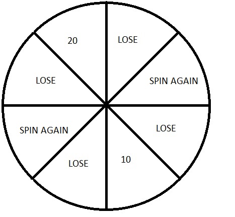
How much would you pay to spin this wheel (the numerical values are prizes):
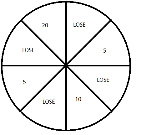
Such games should be analysed using expected average. Imagine playing it 80 times. You expect to hit each of the eight ‘prizes’ ten times:
winnings from 80 plays = 10*20+10*5+10*10+10*5=400,
and so dividing this by 80 we get an expected average of 5. This means, on average, when you play you win 5. Therefore if you intend on playing regularly, if you pay less than €5 you will win on average.
If we divide the above sum by 80 we see:
expected winnings = ![\displaystyle \frac18\cdot 20+\frac18\cdot 5+\frac18\cdot 10+\frac18\cdot 5=\sum_i \mathbb{P}[\text{prize}]\cdot \text{[prize]}](https://s0.wp.com/latex.php?latex=%5Cdisplaystyle+%5Cfrac18%5Ccdot+20%2B%5Cfrac18%5Ccdot+5%2B%5Cfrac18%5Ccdot+10%2B%5Cfrac18%5Ccdot+5%3D%5Csum_i+%5Cmathbb%7BP%7D%5B%5Ctext%7Bprize%7D%5D%5Ccdot+%5Ctext%7B%5Bprize%5D%7D&bg=ffffff&fg=545454&s=0&c=20201002)
This sum here is ‘add up prize by probability of prize’.
When the spinning machine has a ‘spin again’ it is also possible to analyse it. Consider the following:
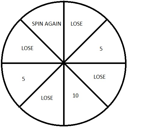
Using the expected winnings equal to ![\sum \mathbb{P}[\text{prize}]\cdot [\text{prize}]](https://s0.wp.com/latex.php?latex=%5Csum+%5Cmathbb%7BP%7D%5B%5Ctext%7Bprize%7D%5D%5Ccdot+%5B%5Ctext%7Bprize%7D%5D&bg=ffffff&fg=545454&s=0&c=20201002)
expected winnings = 
But the spin again prize is the same as the expected winnings so we have, if we denoted by 

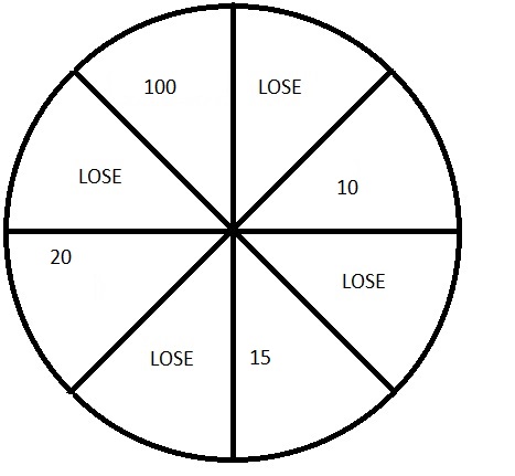
Exercises
Value the following games:

Leave a comment
Comments feed for this article