I am not sure has the following observation been made:

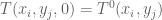
When the Jacobi Method is used to approximate the solution of Laplace’s Equation, if the initial temperature distribution is given by T^0(\mathbf{x}), then the iterations T^{\ell}(\mathbf{x}) are also approximations to the solution, T(\mathbf{x},t), of the Heat Equation, assuming the initial temperature distribution is T^0(\mathbf{x}).

I first considered such a thought while looking at approximations to the solution of Laplace’s Equation on a thin plate. The way I implemented the approximations was I wrote the iterations onto an Excel worksheet, and also included conditional formatting to represent the areas of hotter and colder, and the following kind of output was produced:

Let me say before I go on that this was an implementation of the Gauss-Seidel Method rather than the Jacobi Method, and furthermore the stopping rule used was the rather crude |T^{\ell+1}_{i,j}-T^{\ell}_{i,j}|<\varepsilon.

However, do not the iterations resemble the flow of heat from the heat source on the bottom through the plate? The aim of this post is to investigate this further. All boundaries will be assumed uninsulated to ease analysis.

Discretisation

Consider a thin rod of length L. If we mesh the rod into n pieces of equal length \Delta x=L/n, we have discretised the rod, into segments of length \Delta x, together with ‘nodes’ 0=x_0<\Delta x=x_1<2\Delta x=x_2<\cdots<n\Delta x=L=x_n.

Suppose are interested in the temperature of the rod at a point x\in[0,L], T(x). We can instead consider a sampling of T, at the points x_i:

\displaystyle T(x_i)=T(i\Delta x)=:T_i.

Similarly we can mesh a plate of dimensions W\times H into an n\times m rectangular grid, with each rectangle of area \Delta x\Delta y, where n\Delta x=W and m\Delta y=H, together with nodes x_{i,j}=(i\Delta x,j\Delta y), and we can study the temperature of the plate at a point \mathbf{x}\in[0,W]\times [0,H] by sampling at the points x_{i,j}:

\displaystyle T(x_{i,j})=T(i\Delta x,j\Delta y)=:T_{i,j}.

We can also mesh a box of dimension W\times D\times H into an n_1\times n_2\times n_2 3D grid, with each rectangular box of volume \Delta x\Delta y\Delta z, where n_1\Delta x=W, n_2\Delta y=D, and n_3\Delta z=H, together with nodes x_{i,j,k}=(i\Delta x,j\Delta y,k\Delta z), and we can study the temperature of the box at the point \mathbf{x}\in [0,W]\times [0,D]\times [0,H] by sampling at the points x_{i,j,k}:

\displaystyle T(x_{i,j,k})=T(i\Delta x,j\Delta y,k\Delta z)=:T_{i,j,k}.

Finite Differences

How the temperature evolves is given by partial differential equations, expressing relationships between T and its rates of change.

Consider some real-valued function x\mapsto f(x). Its derivative at x_i — its rate of change with respect to x — is defined as

\displaystyle f'(x_i)=\lim_{\Delta x\rightarrow 0}\left(\frac{f(x_i+\Delta x)-f(x_i)}{\Delta x}\right).

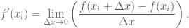
Another way of thinking about this is that we have the following limit as \Delta x\rightarrow 0:

\displaystyle \frac{f(x_i+\Delta x)-f(x_i)}{\Delta x}\longrightarrow f'(x_i),

which implies — by the definition of a limit — that for \Delta x sufficiently close to zero,

\displaystyle \frac{f(x_i+\Delta x)-f(x_i)}{\Delta x}\underset{\text{good}}{\approx} f'(x_i).

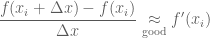
This is known as the forward difference approximation, and here
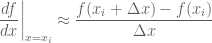
\displaystyle \left.\frac{df}{dx}\right|_{x=x_i}\approx \frac{f(x_i+\Delta x)-f(x_i)}{\Delta x},

will be used.

There is also a backward difference approximation (comes from approaching \Delta x\rightarrow 0 from below):

\displaystyle \left.\frac{df}{dx}\right|_{x=x_i}\approx \frac{f(x_i)-f(x_i-\Delta x)}{\Delta x},

which will be used in the sequel. We will not worry at this time about how accurate or otherwise these approximations are although if we know our calculus, we know they should be good if the second derivative is small near x_i.

Similarly, as \displaystyle f''(x_i) is the derivative of f'(x), i.e.

\displaystyle f''(x)=\frac{d}{dx}\left(f'(x)\right),

we have

\displaystyle \left.\frac{d^2f}{dx^2}\right|_{x=x_i}\approx \frac{f'(x_i+\Delta x)-f'(x_i)}{\Delta x}.

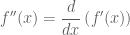
Now use the backwards forward difference approximation on f'(x_i+\Delta x) and f'(x_i):

\displaystyle \approx \frac{\frac{f(x_i+\Delta x)-f(x_i)}{\Delta x}-\frac{f(x_i)-f(x_i-\Delta x)}{\Delta x}}{\Delta x}

\displaystyle =\frac{f(x_i+\Delta x)-2f(x_i)+f(x_i-\Delta x)}{(\Delta x)^2}.

Laplace’s Equation

Rod

The equilibrium temperature distribution on an (insulated) rod, connected to heat sources at x=0 and x=L, of temperatures T_0 and T_1, is given by the solution of the differential equation:

\displaystyle \frac{d^2T}{dx^2}=0, T(0)=T_0, T(L)=T_1.

This can be derived by considering a small length element \Delta x, and considering that, for equilibrium, the heat flowing into \Delta x must equal the heat flowing out of \Delta x (else the heat — and therefore the temperature — in \Delta x is increasing/decreasing).

As a differential equation, it is very easy: it can be antidifferentiated directly. It is probably worth bringing in a small amount of geometric intuition at this point.

Recall that the derivative of T with respect to x is not only the rate of change of T with respect to x, but also slope of the tangent of y=T(x). Therefore, the second derivative of the temperature with respect to distance is the rate of change of the slope of (the tangent to) y=T(x), and, as Laplace’s Equation says, for equilibrium, this is zero, i.e. the rate of change of slope doesn’t change, that is the slope is a constant, that is we have a line (for various technical reasons — let alone physical ones — the second derivative being zero doesn’t give a piecewise-line curve (derivative undefined at jumps)).

Therefore the temperature changes uniformly from T(0)=T_0 to T(L)=T_1, giving solution:

\displaystyle T(x)=\frac{T_1-T_0}{L}x+T_0.

For example, for L=5, T_0=20 and T_1=60:

image1

Plate

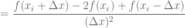
Things are a little more complicated on a plate (uninsulated except at the edges) as the equilibrium temperature distribution T(\mathbf{x}) is now the solution of a partial differential equation, known as Laplace’s Equation:

\displaystyle \frac{\partial^2 T}{\partial x^2}+\frac{\partial^2T}{\partial y^2}=0,    T:\partial(\text{plate})\rightarrow \mathbb{R} given.

Consider a grid point (i,j) with temperature T_{i,j}:

image2

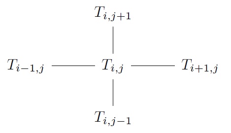
Approximate the second derivatives at x_{i,j} using forward differences:

\displaystyle \left.\frac{\partial^2T}{\partial x^2}\right|_{x_i}\approx \frac{T_{i+1,j}-2T_{i,j}+T_{i-1,j}}{(\Delta x)^2} and

\displaystyle \left.\frac{\partial^2T}{\partial y^2}\right|_{x_i}\approx \frac{T_{i,j+1}-2T_{i,j}+T_{i,j-1}}{(\Delta y)^2}.

If we assume that \Delta x=\Delta y, and substitute these approximations into Laplace’s Equation, we find an equation whose solution approximates T_{i,j}:

\displaystyle \frac{T_{i+1,j}-2T_{i,j}+T_{i-1,j}}{(\Delta x)^2}+ \frac{T_{i,j+1}-2T_{i,j}+T_{i,j-1}}{(\Delta x)^2}=0.

Multiply both sides by (\Delta x)^2 and solve for T_{i,j} to find the Laplace Finite Difference Equation:

\displaystyle T_{i,j}=\frac{T_{i+1,j}+T_{i-1,j}+T_{i,j+1},T_{i,j-1}}{4}=\text{average temperature of adjacent gridpoints}

This approximate equation echoes something called the mean value property for harmonic functions.

Starting with an approximation to each of the T_{i,j}, say all equal to zero, substituting these into the right hand side of this equation gives a better approximation. Iteratively feeding these approximations into the right hand side of this equation gives successively more accurate solutions to the this equation, and this iterative scheme, known as the Jacobi Method, converges to the exact solution of this Laplace Finite Difference Equation.

Heat Equation

The transient temperature distribution on an (insulated) plate, connected to heat sources at \partial(\text{plate}), is given by the solution of the differential equation, known as the Heat Equation:

\displaystyle \frac{\partial T}{\partial t}=k\left(\frac{\partial^2T}{\partial x^2}+\frac{\partial^2T}{\partial y^2}\right), T(x,y,0)\rightarrow \mathbb{R}, T(\partial(\text{plate}),t)\rightarrow \mathbb{R} given.

This can be derived by considering a small area element \Delta x\Delta y, and considering the relationship between the nett heat flowing into \Delta x\Delta y and the resulting change in temperature.

As t\rightarrow \infty,

\displaystyle \frac{\partial T}{\partial t}\rightarrow 0,

that is the temperature does not change, the temperature distribution reaches steady or equilibrium state. Note if the left hand side is equal to zero, the equation reduces to Laplace’s Equation.

This means that if you solve the Heat Equation on a plate using (appropriate) finite differences, the temperatures converge to the same solutions as those of Laplace’s Equation (all else being equal).

The transient temperatures of the plate is a function:

T:[0,W]\times[0,H]\times[0,\infty)\rightarrow \mathbb{R},\,(x,y,t)\mapsto T(x,y,t).

We mesh up the domain using \Delta x=\Delta y but also, for time, \Delta t. Write

T_{i,j}^\ell\approx T(x_i,y_j,t_\ell)=T(i\Delta x,j\Delta y,\ell\Delta t)

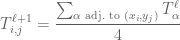
Now use finite differences to approximate the heat equation at (x_i,y_j,t_\ell):

\displaystyle \frac{T^{\ell+1}_{i,j}-T^\ell_{i,j}}{\Delta t}=k\left(\frac{T_{i+1,j}^\ell-2T_{i,j}^\ell+T_{i-1,j}^{\ell}}{(\Delta x)^2}+\frac{T_{i,j+1}^\ell-2T_{i,j}^\ell+T_{i,j-1}^{\ell}}{(\Delta y)^2}\right).

Via \Delta x=\Delta y, this can be written as:

\displaystyle T_{i,j}^{\ell+1}=T_{i,j}^\ell+\frac{k\Delta t}{(\Delta x^2)}\left(-4T_{i,j}^\ell+ \sum_{\alpha\text{ adj. to }(x_i,y_j)}T_{\alpha}^\ell\right),

in short, a formula for the temperature at (x_i,y_j) at time t_\ell=(\ell+1)\Delta t, in terms of the temperature at that point — and the temperatures at the four adjacent points — at the previous time. This is the Heat Finite Difference Equation.

Now, k is a system parameter. The dimensions of the plate are also a system parameter, and essentially \Delta x is determined by the number of internal gridpoints to be considered. The time step \Delta t is basically a free choice.

Note if

\displaystyle\frac{k\Delta t}{(\Delta x^2)}\overset{!}{=}\frac{1}{4},

then the Heat Finite Difference Equation reads:

\displaystyle T_{i,j}^{\ell+1}= \frac{\sum_{\alpha\text{ adj. to }(x_i,y_j)}T_{\alpha}^\ell}{4},

exactly the same as the Laplace Finite Difference Equation!

Therefore, suppose we have a plate with internal gridpoints spaced a distance \Delta x apart, and the plate material parameter is k. Suppose we are interested in the steady state temperature distribution, and our initial approximation to the steady state distribution is given by T^0(x_i,y_j), then using the Laplace Finite Difference Equation, which converges to the steady state solution, also gives the transient temperatures of a plate with initial temperature T(x_i,y_j,0)=T^0(x_i,y_j) but at time steps of:

\displaystyle \Delta t= \frac{(\Delta x)^2}{4k}.

This means that when using the Jacobi Method (without over-relaxation) to approximate the steady state, the intermediate approximations do have physical meaning.

Advertisement