
Consider the symmetric group 


![X\sim \mathrm{Poi}[1]](https://s0.wp.com/latex.php?latex=X%5Csim+%5Cmathrm%7BPoi%7D%5B1%5D&bg=ffffff&fg=545454&s=0&c=20201002)


![\displaystyle \lim_{N\to \infty}\mathbb{P}[\mathrm{fix}_N(\xi_N)=m]=\mathbb{P}[X=m]](https://s0.wp.com/latex.php?latex=%5Cdisplaystyle+%5Clim_%7BN%5Cto+%5Cinfty%7D%5Cmathbb%7BP%7D%5B%5Cmathrm%7Bfix%7D_N%28%5Cxi_N%29%3Dm%5D%3D%5Cmathbb%7BP%7D%5BX%3Dm%5D&bg=ffffff&fg=545454&s=0&c=20201002)
In this note we will look at the distribution in the case where the uniform distribution is conditioned on 
Theorem
Let ![1+\mathrm{Poi}[1]](https://s0.wp.com/latex.php?latex=1%2B%5Cmathrm%7BPoi%7D%5B1%5D&bg=ffffff&fg=545454&s=0&c=20201002)
![\displaystyle \lim_{N\to \infty}\mathbb{P}[\mathrm{fix}_N(\xi_N)=m]=\mathbb{P}[X=m-1]](https://s0.wp.com/latex.php?latex=%5Cdisplaystyle+%5Clim_%7BN%5Cto+%5Cinfty%7D%5Cmathbb%7BP%7D%5B%5Cmathrm%7Bfix%7D_N%28%5Cxi_N%29%3Dm%5D%3D%5Cmathbb%7BP%7D%5BX%3Dm-1%5D&bg=ffffff&fg=545454&s=0&c=20201002)
Proof: What can be shown, ostensibly from stuff from the quantum permutation side of the house is that, where 


the 

![\displaystyle \sum_{t=0}^\infty t^k\mathbb{P}[1+X=t]=\sum_{t=0}^\infty t^k\mathbb{P}[X=t-1]](https://s0.wp.com/latex.php?latex=%5Cdisplaystyle+%5Csum_%7Bt%3D0%7D%5E%5Cinfty+t%5Ek%5Cmathbb%7BP%7D%5B1%2BX%3Dt%5D%3D%5Csum_%7Bt%3D0%7D%5E%5Cinfty+t%5Ek%5Cmathbb%7BP%7D%5BX%3Dt-1%5D&bg=ffffff&fg=545454&s=0&c=20201002)


using the fact that the Bell numbers are the moments of that Poisson distribution and the standard recurrence for the Bell numbers.
Local vs Global Conditioning of Quantum Permutations
In the quantum case we define

where 


Note that when we measure the Haar state with some finite spectrum version of
- the probability of finding an integer number of fixed points is zero, and
- independently of
, the probability of finding more than four fixed points is zero.
In the classical case above when we chose the permutation uniformly from those who fix one, there are two ways of viewing it:
- we pick an element of
- we consider the isotropy subgroup
and choose our permutation from
.
Classically, these are the same thing. In the quantum case these two things can be interpreted differently. The second case is quite clear in the quantum case. For 


The analogue of the uniform distribution on 


I guess this is marginally more interesting than the unshifted version.
Now, what about an analogue of “we pick an element of 

And, it turns out, as above, using stuff from the quantum permutation side of the house:
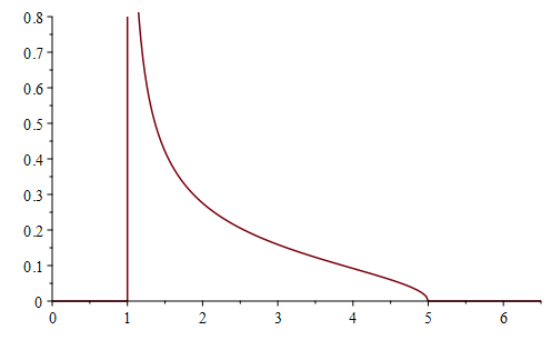
Quite quickly from here we find that the density of the distribution of 

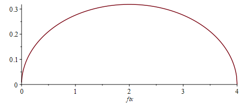
This is so interesting:
- it doesn’t change the support — we still find between 0 and 4 fixed points,
- we have a new symmetry about
, we had another unexpected symmetry here.
- the mean jumps from one to two, that is not unexpected, but
- the mode jumps from zero to two!
- even though we have observed one to one, there can still be less than one fixed point when we measure… and this happens with probability
.
The next obvious question is what happens with:

Epilogue?
So what about this local vs global conditioning? Well, no matter what subsequent measurements are made to
This is not the case with

Leave a comment
Comments feed for this article