I am emailing a link of this to everyone on the class list every week. If you are not receiving these emails or want to have them sent to another email address feel free to email me at jpmccarthymaths@gmail.com and I will add you to the mailing list.

Test

Yes test this Monday morning at 10:00. Any questions send me an email or even better comment below.

Homework

Ye will be getting a homework assignment a lá MS2002 last year. I hope to have more information on this next week.

Tutorial Venue

I have applied to get this changed to WGB G03… I didn’t get everything. The timetable is

  • This week coming, 21 February WGB G03
  •  28 February LL2
  • 7 March LL2
  • 14 March WGB G03
  • 21 March WGB G03
  • 28 March WGB G03

Week 5

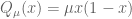
We continued our study of the Logistic Map given by

Q_\mu(x)=\mu x(1-x)

where x\in[0,1] can be interpreted as the proportion of a maximum population with a growth rate \mu\in[0,4]. We found the fixed points of Q_\mu in terms of the growth rate. These were found to be at zero and \displaystyle \frac{\mu-1}{\mu} (the second one only applies when \mu\geq 1; why?). We analysed when zero was attracting/repelling and when \displaystyle \frac{\mu-1}{\mu} was attracting/repelling. We summarised our results in a bifurcation diagram

bifurcation

The green line corresponds to attracting fixed points and the red, dashed line to repelling fixed points. The graph is of fixed points vs \mu.

The fact that there are no attracting fixed points for \mu>3 indicates that the behaviour is more complicated when the growth rate, \mu, gets large. We could have periodic behaviour and perhaps more strange, chaotic behaviour.

We studied therefore the case where \mu=4. We said that for \mu=4Q_\mu is symmetric about x=1/2 and is unimodal. We showed that  Q_4^n has 2^{n-1} branches and hence 2^n period-n points.

We then postulated the existence of more complicated behaviour, chaotic behavior. The first thing we needed was a point with a dense orbit: such a point would necessarily not have any pattern or any periodicity:

dense orbit

What next?

We will finish writing off our definition of what a chaotic dynamical system and do a special study of the tent mapping.

Tutorials

Exercises for Thursday 21 February are to look at the following:

Summer 2011 Question 2(c)

Summer 2010 Question 2(b), (c)

Summer 2009 Question 2(b), 3(d), 4(c)

I understand that ye are busy with the test on Monday but after this I would strongly urge you to look at these problems and also the ones from Week 5

I am emailing a link of this to everyone on the class list every Friday afternoon. If you are not receiving these emails or want to have them sent to another email address feel free to email me at jpmccarthymaths@gmail.ie and I will add you to the mailing list.

Projects

These are finally corrected. I would like to apologise for the inexplicable delay… you are identified by the last five digits of your student number. Remarks below.

S/N Mark Ex 12.5
27898 12.5
29579 12.5
89138 12.5
35809 12
00988 12
05441 12
72936 11.5
31148 11
59663 11
89362 11
19801 10.5
76939 10
55503 10
64923 10
50316 10
56576 9.5
01642 9.5
81431 9.5
28745 9.5
25441 9
11938 9
93481 9
40198 9
37211 9
28575 8.5
30609 8
09341 8
98786 8
04996 7.5
21361 7.5
21967 7
29768 7
00633 7
59593 6.5
84181 6
35726 6
32338 5.5
07743 5.5
30948 5.5
74522 4.5
47692 4.5
93528 4
28475 4
59528 3.5
15585 3.5
71579 3
09658 3
47796 5
64301 5

Remarks

Read the rest of this entry »

Taken from An Invitation to Quantum Groups and Duality by Timmermann.

Let A be a quantum group with a comultiplication \Delta. We make the following definitions. A corepresentation of A on a complex vector space V is a linear map \chi:V\rightarrow V\otimes A that dualises representations with the coassociativity and counit properties:

(I\otimes \Delta)\circ \chi=(\chi\otimes I)\circ \chi, and

(I \otimes\varepsilon)\circ\chi=I.

Now we wish to dualise the terms invariantirreducible, unitary, intertwiner, equivalent, matrix elements. As we want a theory dual to group representation we won’t use Timmermann’s definitions at face value but instead construct them from their group representation counterparts. This might prove difficult. In attempting to dualise group representation theory as quantum group corepresentation theory is ‘everything’ dualised?  Our first term here provides a problem. Do we need an invariant corepresentation or a ‘coinvariant representation’?

Invariant

An invariant subspace of a group representation \Phi:(V,G) is a subspace W\subset V such that

\Phi(w,g)\in W for all w\in W and g\in G.

This means that for the family of linear maps \{\rho(g):g\in G\}W is stable subspace. How this is dualised is important in how we may hope to write a corepresentation as a direct sum of irreducible corepresentations so we need the right definition. Timmermann calls W\subset V invariant if \chi(W)\subset W\otimes A. If we could view the co-representation as a family of endomorphisms on V then we might be able to write down a definition of co-invariant or maybe say that Timmermann’s definition is what we need.

As an example of what we might need to do let \Phi:F(G)\times G\rightarrow G be the regular action of a group and let W\subset be the subspace of constant functions. This set is invariant. Thinking about this yields a definition of co-invariant. 

A subspace W\subset V is co-invariant for \chi if W\otimes A\subset \chi(W).

Timmermann’s definition makes good sense. One is confused between invariant co-representation and co-invariant co-representation. I am guessing that Timmermann’s definition will allow us to do what we want.

Read the rest of this entry »

I am emailing a link of this to everyone on the class list every week. If you are not receiving these emails or want to have them sent to another email address feel free to email me at jpmccarthymaths@gmail.com and I will add you to the mailing list.

Tutorial Venue

I have applied to get this changed to WGB G03… I didn’t get everything. The timetable is

  • This week coming, 14 February LL2
  • Next week, 21 February WGB G03
  •  28 February LL2
  • 7 March LL2
  • 14 March WGB G03
  • 21 March WGB G03
  • 28 March WGB G03

Test

The test will now take place on Monday week February 18. Everything up to but not including section 3.4 in the typeset notes is examinable. We have everything for the test covered. Please find a sample test and the test I gave last year in your typeset notes.

The following theorems from the notes are examinable: Theorem 1 & Theorem 2 (very bottom of page 12 and start of page 13 — called Theorem 1 & 2 on the board). Also the Fixed-Point Factor-Theorem (which was called such on the board. It is not in the notes but is found here https://jpmccarthymaths.com/2012/02/26/ms3011-homework/#comment-331). When I say examinable you should be able to

  • state the theorem
  • prove the theorem
  • understand the theorem and the proof

Learning off the proof letter by letter won’t do you!

Week 5

In week 5 we did a couple of questions that used the theory that we developed in the first few weeks.

Then we began our study of the Logistic Family. We postulated the equation as a model of population growth with two assumptions. We showed how the population could be written as a dynamical system and showed that when the growth-rate parameter \mu=2 then all initial states x_0\in(0,1) converge to the attracting fixed point of Q_2(x)=2x(1-x).

We will continue this study next week.

Exercises

Exercises for Thursday 14 February are to look at the following:

Sample Test & Actual Test in written notes

Autumn 2012: Question 2(a), 3 (a)

Summer 2011: Question 2(a), (b), (d), 4

Summer 2009: Question 4 (a), (b)


I am emailing a link of this to everyone on the class list every Friday afternoon. If you are not receiving these emails or want to have them sent to another email address feel free to email me at jpmccarthymaths@gmail.ie and I will add you to the mailing list.

Tutorials

I am going to take attendance from now on particularly at Friday’s tutorial. If there are more than 15 people at a Friday tutorial then the best-attending surplus will be invited to go to the Tuesday tutorial. There were only 14 at today’s tutorial so the BIS are on their own this Tuesday and all of the Bio are to attend their tutorial on Friday.

Week 1

In week 1 we introduced the idea of a matrix and explored some of the algebra of matrices such as addition, scalar multiplication, transpose and multiplication.

Week 2

In Week 2 we introduced the idea of the inverse of a matrix. If we want to calculate the inverse of a matrix we do the Gauss-Jordan algorithm. Why the Gauss-Jordan algorithm works is answered in the language of elementary matrices and row operations.

Next Week

We see how to use matrix inverses to solve simultaneous equations; e.g.

2x+3y+z=11

x+y+z=6

4x-y+10z=32

Notes

Please find attached.

I am emailing a link of this to everyone on the class list every week. If you are not receiving these emails or want to have them sent to another email address feel free to email me at jpmccarthymaths@gmail.com and I will add you to the mailing list.

Maple Assessment

I have decided to allocate the Maple marks as follows:

  • 5 x Maple Labs @ 2% each
  • Maple Exam @ 5%

This means that if you participate in all of the Maple labs you will have 10%. If you have done this you should be well able for the Maple Exam in Week 12. More information on this in Week 10.

Week 1

In Week 1 we explained the kind of thing that we would be looking at in this module. We did a quick review of integral calculus.

Week 2

In Week 2 we looked at Integration by Parts: this is the start of the new material. In Maple we did some basic plotting, differentiation and integration.

Next Week

We will look at Partial Fractions and possibly start Multivariable Calculus.

Notes

I have given out 13 sets of the notes. I received the E12 from most people: if you didn’t bring it this week you may bring it next week. I now have five more copies of the notes ready for the people who were left without (one week on/off, two day students, one lad who had the money and another lad who was in with me last year). If you did not attend either of the first two lectures please email me so I can another set of notes printed cheers.

I said that to those that I should have had notes for that I would give ye a set of Week 2 notes… here they are: Lecture Two.

I am emailing a link of this to everyone on the class list every week. If you are not receiving these emails or want to have them sent to another email address feel free to email me at jpmccarthymaths@gmail.com and I will add you to the mailing list.

Monday

No Maths on Monday ye have Geotech instead.

Continuous Assessment

You will have 15% tests in Weeks 6 & 11. It would be my intention that the Week 6 Test will cover material from the first four weeks and that the the Week 11 Test would cover material from weeks 5-9. Either way you will receive sample tests and additional information in Week 4 and Week 9 respectively.

Week 1

In the first week we had our introductions and looked at finite difference methods.

Week 2

In the second week we looked at Lagrange Interpolation and Least Squares Curve Fitting.

Next Week

We start Chapter 2: Linear Algebra.

Read the rest of this entry »

I am emailing a link of this to everyone on the class list every week. If you are not receiving these emails or want to have them sent to another email address feel free to email me at jpmccarthymaths@gmail.com and I will add you to the mailing list.

Test

The test will now take place on Monday February 18. Everything up to but not including section 3.4 in the typeset notes is examinable. We have everything for the test covered. Please find a sample test and the test I gave last year in your typeset notes.

Week 4

In week 4 we introduced the idea of a cob-web diagram, which illustrates the dynamics of points near fixed points.

We showed that if we take an iterator function of the form f(x)=mx+c, a line with slope m>0, then the fixed point of this iterator function is either attracting or repelling. 

A fixed point x_f\in S is an attracting fixed point if there exists an interval I containing x_f such that all orbits that begin in I converge to x_f.

A fixed point x_f\in S is a repelling fixed point if there exists an interval I containing x_f such that all orbits that begin in I eventually leave I.

As differentiable functions are approximated well by lines, we argued that if the slope of an iterator function is less than one (although positive) near a fixed point that this fixed point might be attractive.

Read the rest of this entry »

In Group Representations in Probability and Statistics, Diaconis presents his celebrated Upper Bound Lemma for a random walk on a finite  group G driven by \nu\in M_p(G). It states that

\displaystyle \|\nu^{\star k}-\pi\|^2\leq \frac{1}{4}\sum d_\rho \text{Tr }(\widehat{\nu(\rho)}^k(\widehat{\nu(\rho)}^\ast)^k),

where the sum is over all non-trivial irreducible representations of G.

In this post, we begin this study by looking a the (co)-representations of a quantum group A. The first thing to do is to write down a satisfactory definition of a representation of a group which we can quantise later. In the chapter on Diaconi-Fourier Theory here we defined a representation of a group as a group homomorphism

\rho:G\rightarrow GL(V)

While this was perfectly adequate for when we are working with finite groups, it might not be as transparently quantisable. Instead we define a representation of a group as an action

\Phi:V\times G\rightarrow V.

such that the map \rho(g):V\rightarrow V\rho(g)x=\Phi(x,g) is linear.

Read the rest of this entry »

I am emailing a link of this to everyone on the class list every week. If you are not receiving these emails or want to have them sent to another email address feel free to email me at jpmccarthymaths@gmail.com and I will add you to the mailing list.

Story So Far

In the first three weeks we have defined a dynamical system (S,f). It is a set of states S together with an iterator function/ rule of evolution f:S\rightarrow S. We take an initial state/ seed point x_o\in S and examine the orbit of x_0:

\displaystyle \text{orb}(x_0)=\{x_0,x_1,x_2,x_3,\dots\},

where the states x_1,x_2,\dots are produced iteratively by the iterator function:

x_1=f(x_0) and x_n=f(x_{n-1}).

We developed the Logistic Model of Population Growth, and this comprises an important example of a dynamical system which we will examine in more depth a little later on.

Read the rest of this entry »