
I am emailing a link of this to everyone on the class list every Wednesday morning. If you are not receiving these emails or want to have them sent to another email address feel free to email me at jippo@campus.ie and I will add you to the mailing list.
We covered from Proposition 1.4.3 to Proposition 2.1.5 inclusive. Here are the proofs of the product and quotient rules for the calculus of limits.
Problems
You need to do exercises – all of the following you should be able to attempt. Do as many as you can/ want in the following order of most beneficial:
Wills’ Exercise Sheets
Q.8, 9 from http://euclid.ucc.ie/pages/staff/wills/teaching/ms2001/exercise1.pdf
More exercise sheets
Q. 4 from Problems
Past Exam Papers
Q. 1(a), 2 from http://booleweb.ucc.ie/ExamPapers/exams2010/MathsStds/MS2001Sum2010.pdf
Q . 1(a), 2(a) fromhttp://booleweb.ucc.ie/ExamPapers/exams2009/MathsStds/MS2001s09.pdf
Q. 1(a), 2 fromhttp://booleweb.ucc.ie/ExamPapers/exams2009/MathsStds/Autumn/MS2001A09.pdf
Q. 1(a) fromhttp://booleweb.ucc.ie/ExamPapers/exams2008/Maths_Stds/MS2001Sum08.pdf
Q. 1(a), 2(a)(i), (b) fromhttp://booleweb.ucc.ie/ExamPapers/Exams2008/MathsStds/MS2001a08.pdf
Q. 2 fromhttp://booleweb.ucc.ie/ExamPapers/exams2007/Maths_Stds/MS2001Sum2007.pdf
Q. 1, 2(a) fromhttp://booleweb.ucc.ie/ExamPapers/exams2006/Maths_Stds/MS2001Sum06.pdf
Q. 1, 2(a) fromhttp://booleweb.ucc.ie/ExamPapers/exams2006/Maths_Stds/Autumn/ms2001Aut.pdf
Q. 1, 2(a) fromhttp://booleweb.ucc.ie/ExamPapers/Exams2005/Maths_Stds/MS2001.pdf
Q. 1, 2(a) fromhttp://booleweb.ucc.ie/ExamPapers/Exams2005/Maths_Stds/MS2001Aut05.pdf
Q. 1(a), 2(a), 3(b) fromhttp://booleweb.ucc.ie/ExamPapers/exams2004/Maths_Stds/MS2001aut.pdf
Q. 1(a), 2 fromhttp://booleweb.ucc.ie/ExamPapers/exams2004/Maths_Stds/ms2001s2004.pdf
Q. 1(a), 2(a), 3 fromhttp://booleweb.ucc.ie/ExamPapers/exams2003/Maths_Studies/MS2001.pdf
Q. 1(a), 3 fromhttp://booleweb.ucc.ie/ExamPapers/exams2003/Maths_Studies/ms2001aut.pdf
Q. 1, 2(a) fromhttp://booleweb.ucc.ie/ExamPapers/exams2002/Maths_Stds/ms2001.pdf
Q. 1(a), 2(a), 3 fromhttp://booleweb.ucc.ie/ExamPapers/exams2001/Maths_studies/MS2001Summer01.pdf
Q. 1(a), 2 fromhttp://booleweb.ucc.ie/ExamPapers/exams/Mathematical_Studies/MS2001.pdf
Tutorial Quiz Questions
These are not necessarily of exam standard but are more an exercise to help your understanding. The quiz we never did this week as ye actually did some exercises and asked questions.
 of a space
  which we want to examine. Depending on the type of space
  , we can recover and examine many of the properties of
  . When the process/ property
  and
and  we have that
  because
  as the
  lie in the commutative algebra
  .
. — can we examine it’s “underlying space” in the same way?
 considered in the beginning of the previous section. If
  is a group, then
  , if it satisfies the following axioms expressing associativity and unit (
 ),
), , and
, and 
 ,
,  ; and where
  is the identity. As before we have the unital *-homomorphisms
  . Actually, in order to get a representation of
  , i.e.
  for all
  we modify the definition and use
  . (Otherwise we get an anti-representation. But this is a minor point at this stage). In the associated coaction
  the axioms above are turned into the coassociativity and counit properties. These make perfect sense not only for groups but also for quantum groups and we state them at once in this more general setting. We are rewarded with a particular interesting class of quantum Markov chains associated to quantum groups which we call random walks and are the subject of this lecture.
 be finite sets. Any map
  be the *-algebra of complex functions on
  , we have unital *-homomorphisms (
 )
)  They can be put together into a single unital *-homomorphism
 ,
,  ,
, is the indicator function. We get a natural non-commutative generalisation just by allowing the algebras to become non-commutative (
 and
and  be unital C*-algebras and
  a unital *-homomorphism. Here
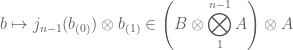
  is the spatial tensor product. Then we can build up the following iterative scheme for
  :
: ,
, 
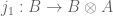 ,
,  .
. stands for
  and is very convenient for writing formulas).
 ,
,  ,
, .
. and
and  are vector spaces, we denote by
  their algebraic tensor product. This is linearly spanned by the elements
  (
( ,
,  ).
). has
has 

 is a bilinear map, where
  and
and  are vector spaces, then there is a unique linear map
  such that
  for all
  are linear functionals on the vector spaces
  on
on 
 ,
,  ,
, , where
  and
and  . If
. If  are linearly independent, then
  . For, in this case, there exist linear functionals
  such that
  . If
. If  is linear, we have
 .
. for arbitrary
  and this shows that all the
  .
. linearly independent, implies that all the
  are zero.
 we should first try
  . If we find that
  except perhaps at
  . Then
 .
. .
. , then
  — which is undefined. However we can cancel an
  above and below… well what we really do is as follows:
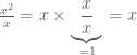 .
. ; i.e. we have that
  for all
  .
.
Recent Comments