Remarks in italics are by me for extra explanation. These comments would not be necessary for full marks in an exam situation. Exercises taken from p.48 of these notes.

Question 1

(i)

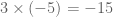
Multiplying the first and last coefficients: $1\times 5=5$ . Now the factors of $5$ are $1\times 5$ . So I want to rewrite the middle term $-4x$ in terms of these:

$x^2-4x-5=x^2+x-5x-5=x(x+1)-5(x+1)=(x+1)(x-5).$

(ii)

Taking out the common factor $x$ : $x(x-2)$ .

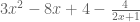
(iii)

Multiplying the first and last coefficients: $15\times6=90$ . The factors of $90$ are $\{90,1\},\{45,2\},\{30,3\},\{18,5\},\{15,6\},\{10,9\}$ . I want to rewrite the middle term $x$ in terms of one of these factors:

$15x^2+10x-9x-6=5x(3x+2)-3(3x+2)=(3x+2)(5x-3)$ .

Question 2

Need to put in long division pictures from a LaTeX file. Answers here:

(i)

$2x+1$ .

(ii)

$x^2-3x+\frac{22}{3}-\frac{40}{3}\frac{1}{3x+1}$ .

(iii)

$x^2-2x-3$

(iv)

$4x^2-6x+9-\frac{25}{2x+3}$

(v)

$x^2-x-6-\frac{40}{2x-5}$

(vi)

$3x^2-8x+4-\frac{4}{2x+1}$

Question 3

By trial and error we are going to see if any of $0,1,2,3,-1,-2,-3,4,-4$ … are a root (recall $k$ is a root of a polynomial $p(x)$ if $p(k)=0$ . Then by the Factor Theorem, $(x-k)$ will be a factor of $p(x)$ .). If we can’t find any like this we might have to be more clever.

(i)

Let $p(x)=2x^3+x^2-8x-4$ .

$p(0)=-4$

$p(1)=2(1)+(1)-8(1)-4=-9$

$p(2)=2(8)+(4)-8(2)-4=16+4-16-4=0\Rightarrow 2$ is a root,

$\Leftrightarrow (x-2)$ is a factor so will divide into $p(x)$ :

Need to put in long division pictures from a LaTeX file. Answer:

$p(x)\div x-2=2x^2+5x+2$ .

Hence

$p(x)=(x-2)(2x^2+5x+2)$ .

Now looking at $2x^2+5x+2$ , I want to rewrite the middle term $5x$ in terms of factors of the product outside terms, $2\times 2=4$ . The factors of $4$ are $\{4,1\},\{2,2\}$ ; hence I rewrite $5x$ as $4x+x$ :

$2x^2+5x+2=2x^2+4x+x+2=2x(x+2)+1(x+2)=(x+2)(2x+1)$ .

Hence

$p(x)=(x-2)(x+2)(2x+1)$ .

(ii)

Let $p(x)=x^3+4x^2+x-6$ .

$p(0)=-6$

$p(1)=(1)+4(1)+(1)-6=0\Rightarrow 1$ is a root,

$\Leftrightarrow (x-1)$ is a factor so will divide into $p(x)$ :

Need to put in long division pictures from a LaTeX file. Answer:

$p(x)\div x-1=x^2+5x+6$ .

Hence

$p(x)=(x-1)(2x^2+5x+6)$ .

Now looking at $x^2+5x+6$ , I want to rewrite the middle term $5x$ in terms of factors of the product outside terms, $1\times 6=6$ . The factors of $4$ are $\{6,1\},\{3,2\}$ ; hence I rewrite $5x$ as $3x+2x$ :

$x^2+5x+6=x^2+3x+2x+6=x(x+3)+2(x+3)=(x+3)(x+2)$ .

Hence

$p(x)=(x-1)(x+3)(x+2)$ .

(iii)

Let $p(x)=3x^3-11x^2+x+15$ .

$p(0)=15$

$p(1)=3(1)-11(1)+(1)+15=8$

$p(2)=3(8)-11(4)+(2)+15=24-44+2+15\neq0$

$p(3)=3(27)-11(9)+3+15=81-99+3+15=0\Rightarrow 3$ is a root,

$\Leftrightarrow (x-3)$ is a factor so will divide into $p(x)$ :

Need to put in long division pictures from a LaTeX file. Answer:

$p(x)\div x-2=3x^2-2x-5$ .

Hence

$p(x)=(x-3)(3x^2-2x-5)$ .

Now looking at $3x^2-2x-5$ , I want to rewrite the middle term $-2x$ in terms of factors of the product outside terms, $3\times (-5)=-15$ . The factors of $-15$ are (will need one plus and one minus) $\{15,1\},\{5,3\}$ ; hence I rewrite $-2x$ as $3x-5x$ :

$3x^2-2x-5=3x^2+3x-5x-5=3x(x+1)-5(x+1)=(x+1)(3x-5)$ .

Hence

$p(x)=(x-3)(x+1)(3x-5)$ .

Question 4

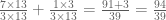
In each case I want each term to have the same denominator; i.e. I can add:

$\frac{3}{71}+\frac{13}{71}=\frac{16}{71}$ ,

but not

$\frac{7}{3}+\frac{1}{13}$ ,

as the denominators do not agree. One quick way to make them agree is to carry out the following:

$\frac{7}{3}.\underbrace{\frac{13}{13}}_{=1}+\frac{1}{13}.\underbrace{\frac{3}{3}}_{=1}$ .

Now, multiplying by $1$ doesn’t change anything but they now share a common denominator, and hence can be added together:

$\frac{7\times 13}{3\times 13}+\frac{1\times 3}{3\times 13}=\frac{91+3}{39}=\frac{94}{39}$ .

This is exactly how we will approach each of these:

$\frac{4x-3}{5}\cdot\frac{3}{3}+\frac{x-3}{3}\cdot \frac{5}{5}=\frac{3(4x-3)+5(x-3)}{15}=\frac{12x-9+5x-15}{15}=\frac{17x-24}{15}$ .

————————————————————————————————————————————————–

$\frac{1}{x-1}\cdot\frac{2x+3}{2x+3}-\frac{2}{2x+3}\cdot\frac{x-1}{x-1}=\frac{1(2x+3)-2(x-1)}{(x-1)(2x+3)}=\frac{2x+3-2x+2}{(x-1)(2x+3)}=\frac{5}{(x-1)(2x+3)}$

————————————————————————————————————————————————–

$\frac{x}{x-1}\cdot\frac{x}{x}+\frac{2}{x}\cdot\frac{x-1}{x-1}=\frac{x^2+2(x-1)}{x(x-1)}=\frac{x^2+2x-2}{x(x-1)}$ .

————————————————————————————————————————————————–

$\frac{1}{x+1}\cdot\frac{2x-1}{2x-1}-\frac{3}{2x-1}\cdot\frac{x+1}{x+1}=\frac{1(2x-1)-3(x+1)}{(x+1)(2x-1)}=\frac{2x-1-3x-3}{(x+1)(2x-1)}=-\frac{x+4}{(x+1)((2x-1))}$

Question 5

In this question we must follow the four steps of doing partial fractions:

Ensure the degree of the top is less than that of the bottom. Divide the bottom into the top if necessary.
Factorise the bottom as far as possible (over the real numbers)
To each factor associate a term in the partial fraction expansion according to rules I-IV
Evaluate the coefficients (well according to the question we won’t do this step)

Step 1: The degree of the top and bottom is 3. Hence we must divide the bottom into the top. Now

$x(x-2)^2=x(x-2)(x-2)=x(x^2-2x-2x+4)=x^3-4x^2+4x$ ;

Need to put in long division pictures from a LaTeX file. Answer:

$x^3-1\div x^3-4x^2+4x=1+\frac{4x^2-4x-1}{x^3-4x^2+4x}$ .

Hence

$\frac{x^3-1}{x(x-2)^2}=1+\frac{4x^2-4x-1}{x(x-2)^2}$ .

Step 2: The bottom is already factorised as much as possible.

Step 3: The factors on the bottom are $x$ and $(x-2)$ (twice). By Rule I, to the linear factor $x$ , we have a term of the form ( $A\in\mathbb{R}$ ):

$\frac{A}{x}$ .

By Rule II, to the repeated linear factor $(x-2)^2$ , we have terms of the form ( $B,C\in\mathbb{R}$ ):

$\frac{B}{x-2}+\frac{C}{(x-2)^2}$ .

Hence we have the partial fraction expansion:

$1+\frac{A}{x}+\frac{B}{x-2}+\frac{C}{(x-2)^2}$

————————————————————————————————————————————————–

Step 1: The degree of the top is two while the degree of the bottom is three $\checkmark$ .

Step 2: We need to factorise $x^3-x^2+x-1$ . To factorise a cubic we use the factor theorem. Let $p(x)=x^3-x^2+x-1$ :

$p(0)=-1$

$p(1)=(1)-(1)+1-1=0\Rightarrow 1$ is a root;

$\Leftrightarrow (x-1)$ a factor. That is $(x-1)$ will divide into $p(x)$ :

Need to put in long division pictures from a LaTeX file. Answer:

$p(x)\div x-1=x^2+1$ .

Hence $p(x)=(x-1)(x^2+1)$ . Now can we factor $x^2+1$ ? We note at this point that we don’t have to factor quadratics as we can use Rules III and IV to associate terms in the partial fraction expansion — however, if we can factorise them we should — it eases calculations later in terms of coefficients, evaluating integrals, and, later, doing inverse Laplace transforms. But can we factorise $x^2+1$ ? Well the roots of $x^2+1$ :

$x^2+1=0\Leftrightarrow x^2=-1$ ,

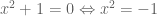
which has no real solutions, hence no real roots, hence no factors of the form $(x-\alpha)$ with $\alpha$ real. $p(x)=(x-1)(x^2+1)$ is as far as we can factorise.

The following little theorem will tell us in general whether or not a quadratic can be factorised:

Theorem

Let $q(x)=ax^2+bx+c$ be a quadratic polynomial over the real numbers (i.e. $a,b,c\in\mathbb{R}$ with $a\neq 0$ ). Then $q(x)$ can be factorised over the real numbers (i.e. written as $a(x-\alpha)(x-\beta)$ for $\alpha,\beta\in\mathbb{R}$ (*)) if and only if $b^2-4ac\geq 0$ .

Proof

Suppose $b^2-4ac\geq 0$ . Now the roots of a quadratic $q(x)=ax^2+bx+c$ are given by:

$x_\pm=\frac{-b\pm\sqrt{b^2-4ac}}{2a}$ .

Now if $b^2-4ac\geq 0$ , then $x_\pm\in\mathbb{R}$ and by the factor theorem both $(x-x_+)$ and $(x-x_-)$ are factors hence

$q(x)=a(x-x_+)(x-x_-)$ .

Suppose on the contrary that $b^2-4ac<0$ . Now $x_{\pm}$ are both complex, $q(x)=a(x-x_+)(x-x_-)$ and hence $q(x)$ cannot be factorised as (*) $\bullet$

Step 3: The factors on the bottom are $x-1$ and $x^2+1$ . By Rule I, to the linear factor $x-1$ , we have a term of the form ( $A\in\mathbb{R}$ ):

$\frac{A}{x-1}$ .

By Rule III, to the quadratic factor $x^2+1$ , we have a term of the form ( $B,C\in\mathbb{R}$ ):

$\frac{Bx+C}{x^2+1}$ .

Hence we have the partial fraction expansion:

$\frac{A}{x-1}+\frac{Bx+C}{x^2+1}$ .

————————————————————————————————————————————————–

Step 1: The degree of the top is two while the degree of the bottom is three $\checkmark$ .

Step 2: By our little ‘quadratic factorisation theorem’, we can test the quadratic term:

$b^2-4ac=(2)^2-4(1)(2)=-4<0\Rightarrow$ further factorisation (over the reals) not possible.

Step 3: The factors on the bottom are $x-1$ and $x^2+2x+2$ . By Rule I, to the linear factor $x-1$ , we have a term of the form ( $A\in\mathbb{R}$ ):

$\frac{A}{x-1}$ .

By Rule III, to the quadratic factor $x^2+2x+2$ we have a term of the form ( $B,C\in\mathbb{R}$ ):

$\frac{Bx+C}{x^2+2x+2}$ .

Hence we have a partial fraction expansion:

$\frac{A}{x-1}+\frac{Bx+C}{x^2+2x+2}$ .

Question 6

This time we will carry out Step 4.

Step 1: The degree of the top is less than that of the bottom $\checkmark$ .

Step 2: Now the bottom has a common factor $x$ , hence:

bottom $=x(x^2-x-2)$ .

Now looking at $x^2-x-2$ , I want to write the middle term, $-x$ , in terms of the factors of the product of the outside terms $1(-2)=-2$ . Now (we will need one plus and one minus) the factors of $-2$ are $\{2,1\}$ . Note that $-x=-2x+x$ . Thus

$x^2-x-2=x^2-2x+x-2=x(x-2)+1(x-2)=(x-2)(x+1)$ .

Hence the bottom is factorised as $x(x-2)(x+1)$ .

Step 3: The bottom has all linear terms, $x,(x-2),(x+1)$ . By Rule I, we have that (for $A,B,C\in\mathbb{R}$ ):

$\frac{x-1}{x^3-x^2-2x}=\frac{A}{x}+\frac{B}{x-2}+\frac{C}{x+1}$ .

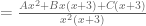
Step 4: Now to evaluate coefficients, we first write the right-hand side as a single fraction (to compare the numerators):

$\frac{A}{x}\cdot\frac{(x+1)(x-2)}{(x+1)(x-2)}+\frac{B}{(x-2)}\cdot\frac{x(x+1)}{x(x+1)}+\frac{C}{(x+1)}\cdot\frac{x(x-2)}{x(x-2)}$

$=\frac{A(x+1)(x-2)+Bx(x+1)+Cx(x-2)}{x(x+1)(x-2)}$ .

Hence we must compare $u(x)= x-1$ with $v(x)= A(x+1)(x-2)+Bx(x+1)+Cx(x-2)$ . Choose test points $x=0,-1,2$ and look at $u(0)=v(0)$ , etc.

$x=0$ ,

$-1=A(1)(-2)+B(0)(1)+C(0)(-2) \Rightarrow 2A=1\Rightarrow A=1/2$ .

$x=-1$ ,

$-2=A(0)(-3)+B(-1)(0)+C(-1)(-3)\Rightarrow 3C=-2\Rightarrow C=-2/3$ .

$x=2$ ,

$1=A(3)(0)+B(2)(3)+C(1)(0)\Rightarrow 6B=1\Rightarrow B=1/6$ .

Hence we have the partial fraction expansion

$\frac{1}{2}.\frac{1}{x}+\frac{1}{6}.\frac{1}{x-2}-\frac{2}{3}.\frac{1}{x+1}$ .

————————————————————————————————————————————————–

Step 1: The degree of the top is zero while the degree of the bottom is 3 $\checkmark$ .

Step 2: Taking out the common factor: $x^3+3x^2=x^2(x+3)$ ; which is factorised fully into linear terms ( $x^2=(x)^2$ ;)).

Step 3: By Rules I (applied to $x+3$ ) and II (applied to $(x)^2$ ) we have the partial fraction expansion:

$\frac{A}{x+3}+\frac{B}{x}+\frac{C}{x^2}$ .

Step 4: First we rewrite the right-hand side as a single fraction:

$\frac{A}{(x+3)}\frac{x^2}{x^2}+\frac{B}{x}\frac{x(x+3)}{x(x+3)}+\frac{C}{x^2}\frac{x+3}{x+3}$

$=\frac{Ax^2+Bx(x+3)+C(x+3)}{x^2(x+3)}$ .

Hence we must compare $u(x)=1$ with $v(x)=Ax^2+Bx(x+3)+C(x+3)$ . Choose test points $x=0,-3,1$ .

$x=0$ ,

$1=A(0)+B(0)(3)+C(3)\Rightarrow 3C=1\Rightarrow C=1/3$ .

$x=-3$ ,

$1=A(9)+B(-3)(0)+C(0)\Rightarrow 9A=1\Rightarrow A=1/9$ .

$x=1$ ,

$1=A(1)+B(1)(4)+C(4)\Rightarrow 1=\frac{1}{9}+4B+\frac{4}{3}$

$\Rightarrow 4B=1-\frac{1}{9}-\frac{4}{3}=\frac{9}{9}-\frac{1}{9}-\frac{12}{9}=-\frac{4}{9}$

$\Rightarrow B=-\frac{1}{9}$ .

Hence we have the partial fraction expansion:

$\frac{1}{9}\cdot\frac{1}{x+3}-\frac{1}{9}\cdot \frac{1}{x}+\frac{1}{3}\cdot\frac{1}{x^2}$ .

————————————————————————————————————————————————–

Step 1: The degree of the top is zero while the degree of the bottom is two $\checkmark$ .

Step 2: The bottom is factored as far as possible $\checkmark$ .

Step 3: Using Rule II we have, for $A,B\in\mathbb{R}$ , partial fraction expansion:

$\frac{A}{x+2}+\frac{B}{(x+2)^2}$ .

Step 4: At this point we should realise that $A$ must be zero and $B$ must be 1. If we carry through the analysis as before we will reach this conclusion also — the function was already written in partial fraction form!

Question 7

In this question we will take the integrand (what is to be integrated), write it in terms of its partial fraction expansion, and then integrate these simpler rational functions term by term.

First we write the integrand in partial fraction form:

$\frac{1}{x^2-4}$ .

Step 1: $\checkmark$ .

Step 2: Difference of two squares! $x^2-4=(x-2)(x+2)$ $\checkmark$ .

Step 3: By Rule I, the integrand has partial fraction expansion:

$\frac{A}{x-2}+\frac{1}{x+2}$ .

Step 4: Write as a single fraction:

$\frac{A}{x-2}\cdot\frac{x+2}{x+2}+\frac{B}{x+2}\cdot\frac{x-2}{x-2}=\frac{A(x+2)+B(x-2)}{(x-2)(x+2)}$ .

Hence we must compare $u(x)=1$ and $v(x)=A(x+2)+B(x-2)$ . Choose test points $x=\pm 2$ .

$x=2$ ,

$1=A(4)+B(0)\Rightarrow 4A=1\Rightarrow A=1/4$ .

$x=-2$ ,

$1=A(0)+B(-4)\Rightarrow 4B=-1\Rightarrow B=-1/4$ .

Hence we have

$\frac{1}{x^2-4}=\frac{1}{4}\cdot\frac{1}{x-2}-\frac{1}{4}\cdot \frac{1}{x+2}$ .

Integration is linear — so we can pull out constants and integrate term-by-term ( $k\in\mathbb{R}$ ):

$I= \int (f(x)+k g(x))\,dx=\int f(x)\,dx+k\int g(x)\,dx$ .

$\Rightarrow \int \frac{1}{x^2-4}\,dx=\frac{1}{4}\int \frac{1}{x-2}\,dx-\frac{1}{4}\int \frac{1}{x+2}\,dx$ .

Now let $u=x-2$ and $v=x+2$ so that $du=dv=dx$ :

$I=\frac{1}{4}\int \frac{du}{u}-\frac{1}{4}\int \frac{dv}{v}=\frac{1}{4}\left[\log |u|-\log|v|\right]+c$ .

Now using the fact that $\log x-\log y=\log (x/y)$ , and then $|x|/|y|=|x/y|$ :

$=\frac{1}{4}\log\left(\frac{|x-2|}{|x+2|}\right)+c=\frac{1}{4}\log\left|\frac{x-2}{x+2}\right|+c$ .

————————————————————————————————————————————————–

Step 1: $\checkmark$ .

Step 2: Well $(8-x)(6-x)=(-(x-8))(-(x-6))=(x-8)(x-6)$ ( $(-a)(-b)=+ab$ ) $\checkmark$ .

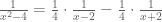
Step 3: We have partial fraction expansion, for $A,B\in\mathbb{R}$ :

$\frac{A}{x-8}+\frac{B}{x-6}$ .

Step 4: Write as a single fraction:

$\frac{A}{x-8}\cdot\frac{x-6}{x-6}+\frac{B}{x-6}\cdot\frac{x-8}{x-8}=\frac{A(x-6)+B(x-8)}{(x-8)(x-6)}$ .

Hence we must compare $u(x)=1$ with $v(x)=A(x-6)+B(x-8)$ . Choose test points $x=6,8$ .

$x=6$ ,

$1=A(0)+B(-2)\Rightarrow B=-1/2$ .

$x=8$ ,

$1=A(2)+B(0)\Rightarrow A=1/2$ .

Hence we have partial fraction expansion:

$\frac{1}{2}\cdot\frac{1}{x-8}-\frac{1}{2}\cdot\frac{1}{x-6}$ .

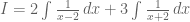
Now integrate:

$I=\frac{1}{2}\int \frac{1}{x-8}\,dx-\frac{1}{2}\int\frac{1}{x-6}\,dx$

Let $u=x-8$ and $v=x-6$ ; then $du=dv=dx$ :

$I=\frac{1}{2}\int\frac{du}{u}-\frac{1}{2}\int\frac{dv}{v}=\frac{1}{2}\left[\log|u|-\log|v|\right]+c$

$=\frac{1}{2}\log\left|\frac{u}{v}\right|+c=\frac{1}{2}\log\left|\frac{x-8}{x-6}\right|+c$ .

————————————————————————————————————————————————–

Step 1: The degree of the top is one while the degree of the bottom is two $\checkmark$ .

Step 2: Again we have a difference of two squares: $x^2-4=(x-2)(x+2)$ .

Step 3: By Rule I we have partial fraction expansion:

$\frac{A}{x-2}+\frac{B}{x+2}$ .

Step 4: Write as a single fraction:

$\frac{A}{x-2}\cdot\frac{x+2}{x+2}+\frac{B}{x+2}\cdot\frac{x-2}{x-2}=\frac{A(x+2)+B(x-2)}{(x-2)(x+2)}$ .

Hence we need to compare $u(x)=5x-2$ with $v(x)=A(x+2)+B(x-2)$ . Choose test points $\pm 2$ .

$x=2$ ,

$5(2)-2=8=A(4)+B(0)\Rightarrow 4A=8\Rightarrow A=2$ .

$x=-2$ ,

$5(-2)-2=-12=A(0)+B(-4)\Rightarrow -4B=-12\Rightarrow B=3$ .

Hence we have partial fraction expansion:

$\frac{2}{x-2}+\frac{3}{x+2}$ .

Now integrating:

$I=2\int \frac{1}{x-2}\,dx+3\int\frac{1}{x+2}\,dx$ .

Let $u=x-2$ and $v=x+2$ ; thus $du=dv=dx$ :

$I=2\int\frac{du}{u}+\int\frac{dv}{v}=2\log |u|+3\log |v|+c$ .

Now using the facts that $\log x^n=n\log x$ , $\log x+\log y=\log xy$ and $|x||y|=|xy|$ (and its extension for powers $|x|^n=|x^n|$ ):

$I=\log|x-2|^2+\log|x+2|^3+c=\log (|x-2|^2|x+2|^3)+c$

$=\log|(x-2)^2(x+2)^3|+c$ .

Comments feed for this article

	J.P. McCarthy on MATH6040: Spring 2022, Week…
	J.P. McCarthy on MATH6040: Spring 2022, Week…
	J.P. McCarthy on MATH7019: Winter 2020, Week…
	J.P. McCarthy on MATH7019: Winter 2020, Week…
	A Sufficient Conditi… on Almost All Trees have Quantum…

MATH6037: Partial Fractions Exercise Solutions

Question 1

(i)

(ii)

(iii)

Question 2

(i)

(ii)

(iii)

(iv)

(v)

(vi)

Question 3

(i)

(ii)

(iii)

Question 4

Question 5

Theorem

Proof

Question 6

Question 7

Recent Comments

Categories

J.P. McCarthy Maths

Leave a comment

Leave a Reply Cancel reply

MATH6037: Partial Fractions Exercise Solutions

Question 1

(i)

(ii)

(iii)

Question 2

(i)

(ii)

(iii)

(iv)

(v)

(vi)

Question 3

(i)

(ii)

(iii)

Question 4

Question 5

Theorem

Proof

Question 6

Question 7

Share this:

Like this:

Related

Recent Comments

Categories

J.P. McCarthy Maths

Leave a comment

Leave a Reply Cancel reply