
Dynamical Systems
A dynamical system is a set of states 


and in general, the next state is got by applying the iterator function:

The sequence of states
is known as the orbit of 

Such dynamical systems are completely deterministic: if you know the state at any time you know it at all subsequent times. Also, if a state is repeated, for example:

then the orbit is destined to repeated forever because


Example: Savings
Suppose you save in a bank, where monthly you receive 

This can be modeled as a dynamical system.
Let 


Now, in the second month, there is interest on all this:
interest in second month 
we also have the 

and it shouldn’t be too difficult to see that how you get from 

Exercise
Use geometric series to find a formula for 
Weather
If quantum effects are neglected, then weather is a deterministic system. This means that if we know the exact state of the weather at a certain instant (we can even think of the state of the universe – variations in the sun affecting the weather, etc), then we can calculate the state of the weather at all subsequent times.
This means that if we know everything about the state of the weather today at 12 noon, then we know what the weather will be at 12 noon tomorrow…
However this isn’t what we tend to experience… instead the weather seems to be very unpredictable.
However this is directly at odds with the contention that the weather is deterministic, which is an assumption underlying how we forecast weather. How do we explain this apparent contradiction?
Sensitivity to Initial Conditions
The first thing we need to understand is sensitivity to initial conditions, more commonly known as Butterfly Effect. What this says is that two initial states, arbitrarily close together, can have very different orbits, and their iterates diverge: that is we can have two initial states 


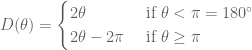
To explain this, suppose for arguments sake that the temperature at a particular point on earth at 12 noon depends only on the temperature at 12 noon on the previous day. The temperature can be modeled as a dynamical system, with some iterator function giving the temperature now in terms of the temperature on the previous day:

Here 


Here we orbits of 

Now this isn’t necessarily a big deal. We can still predict the temperature on subsequent days if we know 
Where do we get 


This measurement challenge is always present for real-life weather forecasters… and sensitivity to initial conditions means we have the following principle:
Any limitation in measuring the weather conditions translates into a limitation of weather forecasting.
Perhaps at a later stage we will describe how real weather forecasters might get around this to a degree.
Chaotic Systems
Systems that display sensitivity to initial conditions are inherently difficult to predict (with the presence or rather inevitability of measurement error).
Topological Mixing
Another way that a system can be ‘chaotic’ is if orbits avoid any periodic pattern. For example, look at this plot of the price of IBM shares:

There doesn’t seem to be any rhyme nor reason: it just looks like… chaos. As written above, an aspect of dynamical systems:
initial state 
is that if a state is ever repeated, then the system will fall into periodic behaviour. If we want a really chaotic orbit, that never repeats itself, then we must have a system with an orbit that never visits the same state twice.
If we have a chaotic orbit (never repeats) that actually gets close to every possible state, then we say we have a dense orbit. A periodic orbit can never be dense: it only contains finitely many distinct states (because it repeats itself) and so cannot get arbitrarily close to every single possible state.
In fact, we can go further and ask that most initial states are chaotic and have dense orbit. This is called topological mixing (basically most orbits never repeat and are… ‘all over the place’).
Density of Periodic Points
In the presence of sensitivity to initial conditions AND topological mixing (‘mad’ lookin’ orbits) there is one more thing that makes a system even harder to predict.
Sensitivity to initial conditions give quantitative differences between two initially close orbits. Quantitative because there is a number that describes that difference:

In truly chaotic systems we want to add some qualitative differences too. We want it to be possible for the orbits of two close initial states 


This is the final signifier of chaos… sort of like mega-sensitivity to initial conditions. For example, starting at a period-three temperature 


There is an initial state
A system that exhibits all three of the following (or maybe just two: there are various definitions) is said to be a chaotic system:
- Sensitivity to Initial Conditions
- Topological Mixing
- Density of Periodic Points
A double pendulum is an example of a chaotic system.
Chaos can exist in very simple systems. Here we show it is present in the following, very simple system.
Doubling Mapping
Let the set of states be given by 


For example, as 

and as 

Model: Doubling Angle
Very similar to this, we have the dynamical system where the set of states is the set of points on the unit circle (given by the angle 


That is you get from one point to the next by doubling the angle… if you go over the 
Start at a given angle and keep doubling the angle basically.
Getting back to the Doubling Mapping (not points on a circle), we will show that this system is chaotic. First let us represent the states slightly differently.
Binary
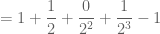
We represent numbers between zero and one by decimals. How this works is as follows. Take the number 

This is the decimal, or base-10, expansion.
We can also consider the binary, or base-two expansion. Note that all decimal digits are between zero and nine (

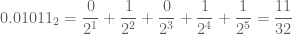
So for example, consider the number between zero and one given in binary by 0.01011. We usually write 
The thing about the Doubling Mapping is that it is very to see what it does to a state when the state is written in binary.
Note first of all that any 


Exercise
Use geometric series to show that:


Now take any state 


noting that:


that is
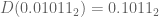
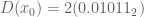
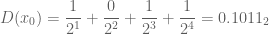
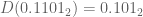
so all the iterator function 
Exercise
Show that where


Any 


that is the first binary digit must be one (with the exception of 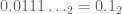


so that
so that, again, the iterator function
Exercises
Show that where

Putting the two exercises together we see that:

Sensitivity to Initial Conditions
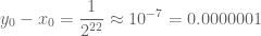
Consider the state:
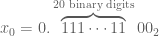
Consider also

Now the difference between these two is very small:
Now apply the doubling mapping to both 20 times (i.e. chop off the first twenty ones:


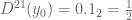
This means that initially the distance between the states is small, 

The initial states
Problems for Friday
- Come up with a seed
- Show that close to every point there is a periodic point.
![x\in [0,1]](https://s0.wp.com/latex.php?latex=x%5Cin+%5B0%2C1%5D&bg=ffffff&fg=545454&s=0&c=20201002)
If we can solve these two problems we have shown that the dynamical system 

1 comment
Comments feed for this article
November 21, 2017 at 2:14 pm
MATH6028: Chaos Theory II | J.P. McCarthy: Math Page
[…] This follows on from this post. […]