
This follows on from this post.
Recall the Doubling Mapping 

At the end of the last post we showed that this dynamical system displays sensitivity to initial conditions. Now we show that it displays topological mixing (a chaotic orbit) and density of periodic points.
First we must talk about periodic points.
Periodic Points
Consider, for example, the initial state 

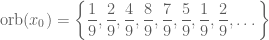
Here we see 
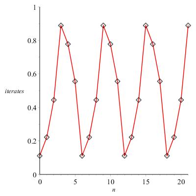
The orbit of 
The orbit of any fraction, e.g. 


and there are only 243 of these and so after 244 iterations, some state must be repeated and so we get locked into a periodic cycle.
If we accept the following:
Proposition
A fraction 

then this is another way to see that fractions are (eventually) periodic. Take for example,
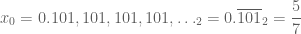
Then, recalling 


we see that if
Proposition
The (eventually) periodic points of 
Exercise
Show that

A Chaotic Orbit
From the above, and the previous post, we know to find an initial state that has a chaotic orbit (never repeating) it cannot be recurring. We also want it to get close to every possible point. Consider the following:
- one digit binaries:
- two digit binaries:
- three digit binaries:
.


Make a state that agrees to these to one, two, three binary places (recall that numbers are close when they agree to a number of binary/decimal places)

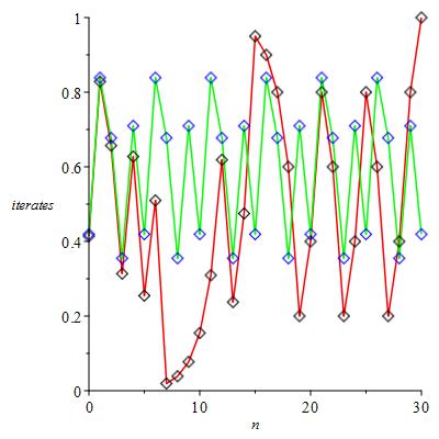
Now this state has a terminating binary expansion and so is a fraction. However note it’s orbit gets close to everything:
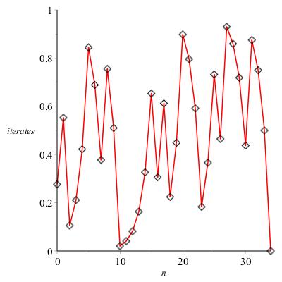
This orbit gets close to everything: draw a horizontal line and some iterate is close to it… but is eventually fixed at 
If instead we keep the pattern going, with all the four digit binaries, the five digit binaries, etc., etc., we get an initial state that is not periodic and gets close to every possible state in 
Such an initial state has a chaotic orbit.
Density of Periodic Points
Have we got close to every state a periodic state. Yes! Take any 

Note that 

This is the density of periodic points and the mega-sensitivity to initial conditions mentioned in the previous post. I believe that 

Therefore
Prediction in the Presence of Chaos
In the real world, measurement come with an error. Suppose, for example, that we measure many aspects of the weather and feed them into our computer models that predict temperature.
Now the problem is, if we think the temperature today is 15.5, and measurement error of 


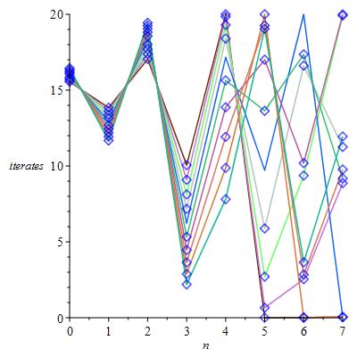
Here we see the orbits of ten initial states close to 


Leave a comment
Comments feed for this article