
You are currently browsing the category archive for the ‘General’ category.
Consider the following question. 


There is a problem with the interpretation and I wouldn’t treat this particular exercise with much importance.
Suppose that


Find the expected average of the profit on a single room. Find the expected average of the profit on 1,000 rooms. Find the probability that the profit on 1,000 rooms is less than 20,000.
Solution : The expected average of a variable is given by:
![\mathbb{E}[X]=\sum_ix_i\mathbb{P}[X=x_i]=\sum_ix_ip_i](https://s0.wp.com/latex.php?latex=%5Cmathbb%7BE%7D%5BX%5D%3D%5Csum_ix_i%5Cmathbb%7BP%7D%5BX%3Dx_i%5D%3D%5Csum_ix_ip_i&bg=ffffff&fg=545454&s=0&c=20201002)
Now expected average is linear:
![\mathbb{E}[X+\lambda Y]=\sum_i(x_i+\lambda y_i)p_i=\sum_{i}x_ip_i+\lambda\sum_i y_i p_i](https://s0.wp.com/latex.php?latex=%5Cmathbb%7BE%7D%5BX%2B%5Clambda+Y%5D%3D%5Csum_i%28x_i%2B%5Clambda+y_i%29p_i%3D%5Csum_%7Bi%7Dx_ip_i%2B%5Clambda%5Csum_i+y_i+p_i&bg=ffffff&fg=545454&s=0&c=20201002)
![=\mathbb{E}[X]+\lambda\mathbb{E}[Y]](https://s0.wp.com/latex.php?latex=%3D%5Cmathbb%7BE%7D%5BX%5D%2B%5Clambda%5Cmathbb%7BE%7D%5BY%5D&bg=ffffff&fg=545454&s=0&c=20201002)
Introduction
This is just a short note to provide an alternative way of proving and using De Moivre’s Theorem. It is inspired by the fact that the geometric multiplication of complex numbers appeared on the Leaving Cert Project Maths paper (even though it isn’t on the syllabus — lol). It assumes familiarity with the basic properties of the complex numbers.
Complex Numbers
Arguably, the complex numbers arose as a way to find the roots of all polynomial functions. A polynomial function is a function that is a sum of powers of 

Definition
Let 


is a polynomial of degree 
In many instances, the first thing we want to know about a polynomial is what are its roots. The roots of a polynomial are the inputs 
Theorem: Cauchy-Schwarz Inequality
Let 


Proof : Consider the following quadratic function 

Note at this point that 


That is 


Now take square roots (remembering 

With the new Project Maths programme being developed as we speak, diligent students might like to know which proofs are examinable under the new syllabus so they know which to look at.
It can be difficult to sift through the syllabi at projectmaths.ie but I have gone through them and here are the proofs required.
I’m giving a talk in Blackrock Castle Observatory on October 7. See the link for more details.
http://www.bco.ie/2011/09/first-fridays-at-the-castle-celebrating-50-years-of-human-spaceflight/
The Average
The average or the mean of a finite set of numbers is, well, the average. For example, the average of the (multiset of) numbers 

When we have some real-valued variable (a variable with real number values), for example the heights of the students in a class, that we know all about — i.e. we have the data or statistics of the variable — we can define it’s average or mean.
Definition
Let 


In Leaving Cert Maths we are often asked to differentiate from first principles. This means that we must use the definition of the derivative — which was defined by Newton/ Leibniz — the principles underpinning this definition are these first principles. You can follow the argument at the start of Chapter 8 of these notes:
https://jpmccarthymaths.com/wp-content/uploads/2010/07/lecture-notes.pdf,
to see where this definition comes from, namely:

This is intended to be the subject of a short postgraduate talk in UCC. At times there will be little attempt at rigour — mostly I am just concerned with ideas, motivation and giving a flavour of the philosophy. Also it is fully possible that I have got it completely wrong in my interpretation!
Introduction
It is a theme in mathematics that geometry and algebra are dual:

Arguably this theme began when Descartes began to answer questions about synthetic geometry using the (largely) algebraic methods of coordinate geometry. Since then this duality has been extended and refined to consider:

Here a space is a set of points with some additional structure, and the idea is that for a given space, there will be a canonical algebra of functions on the space. For example, given a compact, Hausdorff topological space 
Suppose we want to maximise (or minimise) the linear function 

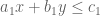

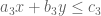
In general, the solution set of these inequalities will be a triangular sea of 
 The points


A short note covering integration for Leaving Cert maths.
(Please note that the proof of the Fundamental Theorem of Calculus inside isn’t quite correct. We need the Mean Value Theorem to prove it but the one in here is just for illustrative purposes.)

Recent Comments