
Remarks in italics are by me for extra explanation. These comments would not be necessary for full marks in an exam situation. Exercises taken from https://jpmccarthymaths.wordpress.com/2011/02/01/math6037-general-information/
Question 1
(a)
Now:


hence:
![\int_0^1 (2x+5)\,dx=\left[x^2+5x\right]_0^1 =(1^2+5(1))-(0^2+5(0))=6](https://s0.wp.com/latex.php?latex=%5Cint_0%5E1+%282x%2B5%29%5C%2Cdx%3D%5Cleft%5Bx%5E2%2B5x%5Cright%5D_0%5E1+%3D%281%5E2%2B5%281%29%29-%280%5E2%2B5%280%29%29%3D6&bg=ffffff&fg=545454&s=0&c=20201002)
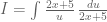
(b)
There is no obvious anti-derivative and there is no obvious manipulation hence we are looking for the function-dervative pattern to make a substitution (or else use the LIATE rule). Notice that the top is the derivative of the bottom. Hence we will let 
Let 


Now put everything back into the integrand, suppressing the limits:
![=\int \frac{du}{u}=\ln u =[\ln (x^2+5x+1)]_0^1](https://s0.wp.com/latex.php?latex=%3D%5Cint+%5Cfrac%7Bdu%7D%7Bu%7D%3D%5Cln+u+%3D%5B%5Cln+%28x%5E2%2B5x%2B1%29%5D_0%5E1&bg=ffffff&fg=545454&s=0&c=20201002)

Now, what do we have to raise 


 (*)
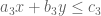
(*) , find the solution to the homogeneous system,
  :
: ,
, .
. on a set
  . Suppose
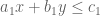

 and
and  :
:
 are the extreme points on
  is maximised at
  .
. be a compact Hausdorff space and
  a Hilbert Space. A spectral measure
  relative to
  is a map from the
  -algebra of all Borel sets of
  such that
 ,
,  ;
; for all Borel sets
  of
of  , the function
  , is a regular Borel complex measure on
  is a measure defined on Borel sets. If every Borel set in
  is inner and outer regular if
 , and
, and
 the Banach space of all regular Borel complex measures on
  the C*-algebra of all bounded Borel-measurable complex-valued functions on
 is the set of unit vectors.
 is a finite-rank projection on
  is finite dimensional. To see this, write
 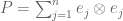 , where
  . If
. If  , then
 , (
, ( ) (*), and therefore is finite dimensional.
Recent Comments