A Poker Hack
I told this story in class on Friday. I wasn’t sure if it was true but it appears that it is.
Texas Hold’Em Poker
‘Texas‘ is a poker game where a number of players sit around a table. Two cards are dealt to each player. There after follows a round of betting, the reveal of three more cards (the flop), more betting, another card (the turn), another round of betting, another card (the river), and another round of betting:

What we are interested in is what happens after all this, before another hand is dealt?
The deck is shuffled.
A shuffle is required to mix up the deck. Here we used three terms: deck, shuffle, mixed up. These can all be given a precise mathematical realisation (see the introduction here for more). Mixed up means ‘close to random’. Here let me introduce a mathematical realisation of random:
If one is handed a deck of cards, face down, and if each possible order of
the cards is equally possible then the deck is considered random.
Note there are  possible orders that a deck can be in so when a deck is random the probability that a deck is in a specific order is
 .
.
One popular method of shuffling cards is the riffle shuffle. In a remarkable 1992 paper by Bayer & Diaconis, with a really cool name: Trailing the Dovetail Shuffle to Its Lair, it is shown that seven riffle shuffles are necessary and sufficient to get a deck close to random:

Here we see  , distance to random, plotted against
  , number of shuffles. After five shuffles the deck is still far from random, but then there is a fairly abrupt convergence to random. After seven shuffles the distance to random is less than
  .
.
So the idea is after, say, ten shuffles (or, equivalently, about ten rounds of hands), the deck is mixed up or close to random: each of the 52! orders are approximately likely.
Read the rest of this entry »

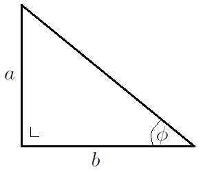
for
(relative velocity example with
below)
without the use of calculus


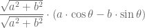


 and
and  , and they appear to have a straight-line relationship, then the
 , said
  days after January 1, and the sales,
  , on that day: for each value of
  m.
m.
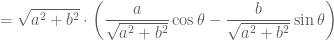
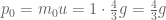
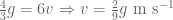
 . Alternatively, we can use Conservation of (Mechanical) Energy.
 , at its maximum height, the 1 kg mass has potential energy and no kinetic energy:
 .
. ,
, :
: .
. :
: .
. .
. .
.
Recent Comments