Dynamical Systems
A dynamical system is a set of states  together with an iterator function
  which is used to determine the next state of a system in terms of the previous state. For example, if
  is the initial state, the subsequent states are given by:
 ,
,

 ,
,
and in general, the next state is got by applying the iterator function:
 .
.
The sequence of states
is known as the orbit of  and the
  are known as the iterates.
Such dynamical systems are completely deterministic: if you know the state at any time you know it at all subsequent times. Also, if a state is repeated, for example:

then the orbit is destined to repeated forever because
 ,
,
 , etc:

Example: Savings
Suppose you save in a bank, where monthly you receive  interest and you throw in
  per month, starting on the day you open the account.
This can be modeled as a dynamical system.
Let  be the set of euro amounts. The initial amount of savings is
  . After one month you get interest on this:
  , you still have your original and you are depositing a further €50, so the state of your savings, after one month, is given by:
 .
.
Now, in the second month, there is interest on all this:
interest in second month  ,
,
we also have the  from the previous month and we are throwing in an extra €50 so now the state of your savings, after two months, is:
 ,
,
and it shouldn’t be too difficult to see that how you get from  is by applying the function:
 .
.
Exercise
Use geometric series to find a formula for  .
.
Weather
If quantum effects are neglected, then weather is a deterministic system. This means that if we know the exact state of the weather at a certain instant (we can even think of the state of the universe – variations in the sun affecting the weather, etc), then we can calculate the state of the weather at all subsequent times.
This means that if we know everything about the state of the weather today at 12 noon, then we know what the weather will be at 12 noon tomorrow…
Read the rest of this entry »


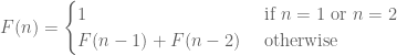
 satisfies the recurrence relation
 ,
, .
. ,
, and
and  , prove that for large
  :
: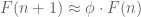
 .
. .
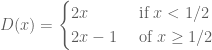
. given by:
 . The orbit of
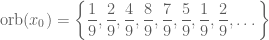
 repeats itself and so gets ‘stuck’ in a repeating pattern:
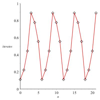
 .
. , must be periodic, because
  is either equal to
  of
of  and so the orbit consists only of states of the form:
 ,
, has a recurring binary expansion:
 ,
,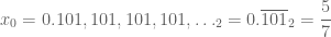 .
. be constants. Let
  be a sequence of real numbers with the following recursive definition:
 .
.
 .
. .
. is the sum of the first


 .
. , find a formula for the geometric series
 .
. .
.


 .
. under
under  .
. .
. has the binary representation
 ,
, and
and  .
.![y, z \in [0, 1]](https://s0.wp.com/latex.php?latex=y%2C+z+%5Cin+%5B0%2C+1%5D&bg=ffffff&fg=545454&s=0&c=20201002) such that
such that  and
and  agree to 5 binary digits but
  and
and  differ in the first binary digit for some
  .
.![w \in [0, 1]](https://s0.wp.com/latex.php?latex=w+%5Cin+%5B0%2C+1%5D&bg=ffffff&fg=545454&s=0&c=20201002) have a binary representation beginning
have a binary representation beginning  . Find a period-5 point
  of
of  and
and ![\delta \in [0, 1]](https://s0.wp.com/latex.php?latex=%5Cdelta+%5Cin+%5B0%2C+1%5D&bg=ffffff&fg=545454&s=0&c=20201002) such that there are iterates of
such that there are iterates of  ,
,  , with
  , that agree with 0.111 , 0.101, and 0.010, to three binary
 . Where
 ![[0,1]](https://s0.wp.com/latex.php?latex=%5B0%2C1%5D&bg=ffffff&fg=545454&s=0&c=20201002) is the set of states, and
is the set of states, and ![f:[0,1]\rightarrow [0,1]](https://s0.wp.com/latex.php?latex=f%3A%5B0%2C1%5D%5Crightarrow+%5B0%2C1%5D&bg=ffffff&fg=545454&s=0&c=20201002) the iterator function, by looking at the first seven iterates of
the iterator function, by looking at the first seven iterates of  and
and  , show that this dynamical system displays sensitivity to initial conditions [HINT:4*ANS*(1-ANS)]
 ). I strongly advise you that attending tutorials alone will not be sufficient preparation for this test and you will have to
  and
and  respectively lie on a smooth horizontal table.
 and
and  respectively.
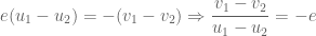
 , the coefficient of restitution
 .
.
 and
and  be the velocities of the smaller respectively larger sphere after collision. Note that the initial velocity of the larger sphere is minus

 .
. ,
,
 ,
, ,
, .
. .
. . If
. If  and so
 ;
;
Recent Comments