
I am emailing a link of this to everyone on the class list every week. If you are not receiving these emails or want to have them sent to another email address feel free to email me at jpmccarthymaths@gmail.com and I will add you to the mailing list.
Continuous Assessment Results
You are identified by the last four digits of your student number. The first column is your Test 1 result while the second is your Maple Labs participation. The third is your Maple Test Mark out of 5. The fourth is your continuous assessment mark out of 30. The last is the percentage you must have on the final to pass. If you have any issues with this please email me.
| Student Number | Test | Maple Labs | Maple Test | CA Mark | Pass |
| 8272 | 93 | 10 | 5 | 28.95 | 15.79 |
| 4673 | 90 | 10 | 3 | 26.5 | 19.29 |
| 1054 | 78 | 10 | 4 | 25.7 | 20.43 |
| 9455 | 65 | 10 | 5 | 24.75 | 21.79 |
| 0902 | 70 | 10 | 3 | 23.5 | 23.57 |
| 2344 | 61 | 10 | 3 | 22.15 | 25.50 |
| 2352 | 58 | 10 | 2 | 20.7 | 27.57 |
| 4346 | 28 | 10 | 3 | 17.2 | 32.57 |
| 3152 | 40 | 10 | 1 | 17 | 32.86 |
| 2343 | 25 | 10 | 3 | 16.75 | 33.21 |
| 2351 | 15 | 8 | 3 | 13.25 | 38.21 |
| 2345 | 28 | 6 | 3 | 13.2 | 38.29 |
| 4674 | 48 | 4 | 0 | 11.2 | 41.14 |
| 3150 | 25 | 6 | 0 | 9.75 | 43.21 |
| 1215 | 0 | 6 | 2 | 8 | 45.71 |
| 8171 | 30 | 0 | 0 | 4.5 | 50.71 |
Study
Please feel free to ask me questions via email or even better on this webpage — especially those of us who struggled in the test.
Please find a reference for some of the prerequisite material here.
Week 12
We finished our work on Laplace Methods and looked at the general solution of the damped harmonic oscillator. The following is the correct way to categorise over and underdamping:
Damped Harmonic Oscillator Analysis
The differential equation
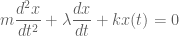
as discussed on page 154 is the equation of a damped harmonic oscillator. There are three behaviours. One way to analyse these is to define the following parameters


and follow the analysis as per the notes. However last night 8 May we outlined an even easier analysis.
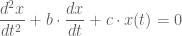
First write the differential equation as it will be on your exam paper
Now find the Laplace Transform of the solution. It will look like

Now there are three cases depending on whether 

Underdamping 
In this case the roots are complex: no real roots implying no real factors hence we must complete the square

which is composed of shifted sines and cosines when we transform it back

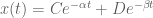
Overdamping 
In this case the roots are real and distinct so we have two factors and hence a partial fraction expansion like this:

which is composed of two exponentially decaying terms when we transform back.
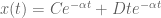
Critical Damping 
In this case the root are real and repeated hence we have repeated real factors and hence a partial fraction expansion like this:

which is composed of an exponentially decaying term and (before transforming) a shifted 
In Conclusion
If you are asked to analyse a damped harmonic oscillator of the form

then you have three options:
- Calculate
. Over-zero = Over-damping, Under-zero = Under-damping and Equal Zero = Critical-damping
- Calculate
and
as described on page 154 of the notes and compare. It is actually equivalent to method 1. In the Laplace marking scheme handout a damped harmonic oscillator is analysed using this method.
- Solve the differential equation using Laplace Methods and see which behaviour the solution corresponds to.
Week 13
We will hold a review tutorial on Wednesday 8 May in the usual room. First off, the layout of your exam is the same as Winter 2012: do question one worth 50/100 and two out of questions two, three, four; each worth 25/100.
I will field any questions ye might have at this time and if there are no questions we will do the exam paper from Autumn 2012.
Formulae to Learn?
Somebody asked me for a list of formulae that ye might need that are not on the tables. I would put the following on that list:
- The Midpoint Rule Formula Here
One could include
- The Differential; if
then

There are a number of others such as 
Math.Stack Exchange
If you find yourself stuck and for some reason feel unable to ask me the question you could do worse than go to the excellent site math.stackexchange.com. If you are nice and polite, and show due deference to these principles you will find that your questions are answered promptly. For example this question about completing the square.

6 comments
Comments feed for this article
May 8, 2013 at 12:12 pm
Student 36
I tried to do the Autumn Paper from 2012 and was just wondering could you have a look and let me know If the answers are right.
No detail needed – yes or no is fine – Ill go back to the drawing board if wrong.
Q1(a).
 .
.
Using
comparing coefficients I get
Q1(b) . I work on getting a shifted cosine & as a result a shifted sine by +/- 3 then * & / 4
Completing the square I get
Leaving me with of the above giving me
Q1(c)(i)
Although probably longer can this be done by saying the denominator is and putting a constant over each and compare coefficients. It works but would it in all cases. Of course it only works if the answer is right.
Q1(c)(ii)
Q1(c)(iii)
Q1(d)
Q1(e)
351.9346 using 0.25,0.75,1.25,1.75,2.25,2.75
Q2 (a)
13.40 by evaluating from from 0 to 2.
Q2 (b)
Using the definition as instructed ended up with
Took me a while to work through it with a lot of workings – made me contemplate not doing question 2. You make it look too easy in notes for winter 2012 so maybe just more practice needed here
Q2 (c)
Struggled here – brain was tired after 2b – any tips??
Q3 (a)
From advice worked with calculating and
and  where
where  stating underdamping.
Looking at your expected answers was slightly concerned not to see a .
.
How do you determine the period & duration of oscillation? – Just for info
Q3 (b)
510 mm /s from
Q4 (a) (i)
Not attempted this exercise
Q4 (a) (ii)
Q4 (b)
5.77 @ 0.9 working with
Q4 (c)
1.3072
Appreciate any feedback.
May 8, 2013 at 4:29 pm
J.P. McCarthy
No bother. You can use Maple to check answers also.
Q. 1(a) — correct
Q. 1(b) — correct
Q. 1(c) (i) — is it not ?
?
Q. 1(c) (ii) — correct
Q. 1(c) (iii) — not quite. A partial fraction expansion gives
Q. 1(d) — correct.
Q. 1(d) — I don’t know what happened to you here… The answer is 0.8862.
Q. 2(a) — Your anti-derivative is correct but not the evaluation. The answer is .
.
Q. 2(b) — hard yes but important if you are progressing on
Q. 2 (c) (i) — first shift theorem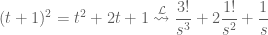 . However the first shift theorem gives
Q. 2 (c) (ii) — use the identity .
.
Q. 3 (a) — should it be of that? The lack of a cosine term is fine and will always happen when
  (why?)
Q. 3 (b) — mighty stuff considering that we never covered it in class!! You have it sussed out anyway… take your equation and ‘divide’ by and that is basically it.
Q. 4 (a) (i) — write it as and do two Chain Rules.
Q. 4 (a) (ii) — correct.
Q. 4 (b) — correct
Q. 4 (c) — correct
Regards,
J.P.
May 10, 2013 at 10:36 am
Student 39
Just looking at Eulers method and just wondering how is transformed to the
  . If you could show me Q. 3 as well page 107 of notes
Many thanks.
May 10, 2013 at 10:42 am
J.P. McCarthy
For Euler’s method the is the derivative/slope/
 /
/ /etc. So we must find
  on it’s own. I would say that both the
  and the
  is in the way so add
  and subtract
  to both sides to get rid:
morryah,
Regarding question 3, the answer given there is certainly wrong… see here https://jpmccarthymaths.com/2013/03/23/math6037-weeks-7-8/#comment-507
Regards.
J.P.
May 13, 2013 at 8:34 am
Student 40
Hey J.P.,
If u get a chance could u show me how to get the laplace transform of .
.
Thanks
May 13, 2013 at 8:42 am
J.P. McCarthy
The issue here is that we have no product rule or chain rule for doing Laplace Transforms. The Laplace Transform is, however, linear and this means that we are good at handling sums.
Therefore if we could write as a sum then we would be away with it. Now there are two ways to do that. One is to use the Binomial Theorem but at this stage if you don’t know what that is you should just multiply out as follows:
Now we can transform all of these using
which is on the Laplace tables. Thus we have
Regards,
J.P.