
In this short note we will explain why we multiply matrices in this “rows-by-columns” fashion. This note will only look at 
First of all we need some objects. Consider the plane 


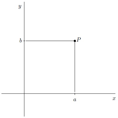
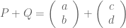
We have two basic operations with points in the plane. We can add them together and we can scalar multiply them according to, if 


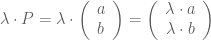
Objects in mathematics that can be added together and scalar-multiplied are said to be vectors. Sets of vectors are known as vector spaces and a feature of vector spaces is that all vectors can be written in a unique way as a sum of basic vectors.
In the case of the plane 


One of the first things to do when an algebraic structure is defined, in this case the plane, is to consider functions on it. A function 


Of particular interest are linear maps. A linear map is a function between two vector spaces that preserves the operations of vector addition and scalar multiplication. In the case of functions 


shows that a linear map is defined what it does to the basis vectors. Suppose that a linear map is defined, for scalars 


then we see that


Now it turns out that all this information can be encoded by a matrix 


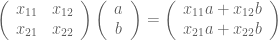
If we take matrix multiplication to be as we define it then multiplying this out we see that the two of these are the same thing:

Therefore two-by-two matrices are actually functions in the sense that every linear map
for some 
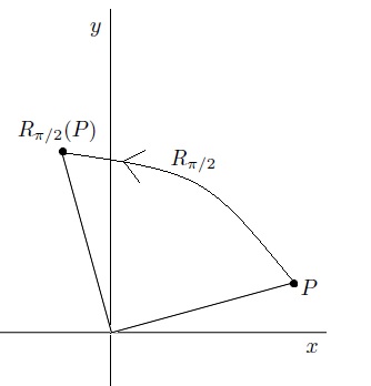
Another notation for 


We can compose two functions to produce another. For example, consider two linear maps 


–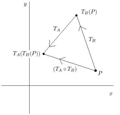
Now this composition is a function in itself, sending 

Now there are two questions. The map 


Let us write 
![[a_{ij}]](https://s0.wp.com/latex.php?latex=%5Ba_%7Bij%7D%5D&bg=ffffff&fg=545454&s=0&c=20201002)
![[b_{ij}]](https://s0.wp.com/latex.php?latex=%5Bb_%7Bij%7D%5D&bg=ffffff&fg=545454&s=0&c=20201002)

and so


Some careful inspection shows that this is nothing but, where 


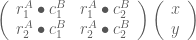
where this 

So the reason that we multiply matrices why we do is that the matrix product 

6 comments
Comments feed for this article
October 5, 2017 at 9:18 am
MATH6040: Winter 2017, Week 4 | J.P. McCarthy: Math Page
[…] at Matrix Inverses — “dividing” for Matrices. This allowed us to solve matrix equations. Here find a note that answers the question: why do we multiply matrices like we […]
February 8, 2018 at 8:07 am
MATH6038: Spring 2018, Week 2 | J.P. McCarthy: Math Page
[…] For those of you interested in the why when it comes to matrix multiplication, have a look here. […]
October 4, 2018 at 9:25 am
MATH6040: Winter 2018, Week 4 | J.P. McCarthy: Math Page
[…] at Matrix Inverses — “dividing” for Matrices. This will allow us to solve matrix equations. Here find a note that answers the question: why do we multiply matrices like we […]
February 20, 2019 at 10:21 am
MATH6040: Spring 2019, Week 4 | J.P. McCarthy: Math Page
[…] Inverses — “dividing” for Matrices. This will allow us to solve matrix equations. Here find a note that answers the question: why do we multiply matrices like we […]
October 3, 2019 at 9:56 am
MATH6040: Winter 2019, Week 4 | J.P. McCarthy: Math Page
[…] to work and moments and began Chapter 2: Matrices. We did some examples of matrix arithmetic. Here find a note that answers the question: why do we multiply matrices like we […]
February 19, 2020 at 8:55 am
MATH6040: Spring 2020, Week 4 | J.P. McCarthy: Math Page
[…] Here find a note that answers the question: why do we multiply matrices like we do? […]