You are currently browsing the category archive for the ‘Quantum Groups’ category.

In Group Representations in Probability and Statistics, Diaconis presents his celebrated Upper Bound Lemma for a random walk on a finite  group G driven by \nu\in M_p(G). It states that

\displaystyle \|\nu^{\star k}-\pi\|^2\leq \frac{1}{4}\sum d_\rho \text{Tr }(\widehat{\nu(\rho)}^k(\widehat{\nu(\rho)}^\ast)^k),

where the sum is over all non-trivial irreducible representations of G.

In this post, we begin this study by looking a the (co)-representations of a quantum group A. The first thing to do is to write down a satisfactory definition of a representation of a group which we can quantise later. In the chapter on Diaconi-Fourier Theory here we defined a representation of a group as a group homomorphism

\rho:G\rightarrow GL(V)

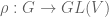
While this was perfectly adequate for when we are working with finite groups, it might not be as transparently quantisable. Instead we define a representation of a group as an action

\Phi:V\times G\rightarrow V.

such that the map \rho(g):V\rightarrow V\rho(g)x=\Phi(x,g) is linear.

Read the rest of this entry »

Let G be a group and let A:=C^*(G)  be the C*-algebra of the group G. This is a C*-algebra whose elements are complex-valued functions on the group G. We define operations on A in the ordinary way save for multiplication

\displaystyle (fg)(s)=\sum_{t\in G}f(t)g(t^{-1}s),

and the adjoint f^*(s)=\overline{f(s^{-1})}. Note that the above multiplication is the same as defining \delta_s\delta_t=\delta_{st} and extending via linearity. Thence A is abelian if and only if G is.

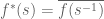
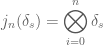
To give the structure of a quantum group we define the following linear maps:
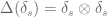
\Delta:A\rightarrow A\otimes A\Delta(\delta_s)=\delta_s\otimes\delta_s.

\displaystyle \varepsilon:A\rightarrow \mathbb{C}\varepsilon(\delta_s)=1.

S:A\rightarrow AS(\delta_s)=\delta_{s^{-1}}.

The functional h:A\rightarrow \mathbb{C} defined by h=\mathbf{1}_{\{\delta_e\}} is the Haar state on A. It is very easy to write down the j_n:

\displaystyle j_n(\delta_s)=\bigotimes_{i=0}^n\delta_s.

To do probability theory consider states \varepsilon,\,\phi on A and form the product state:

\displaystyle \Psi=\varepsilon\otimes\bigotimes_{i=1}^\infty \phi.

Whenever \phi is a state of A such that \phi(\delta_s)=1 implies that s=e, then the distribution of the random variables j_n converges to h.

At the moment we will use the one-norm to measure the distance to stationary:

d(\Psi\circ j_n,h)=\|\Psi\circ j_n-h\|_1.

A quick calculation shows that:

d(\Psi\circ j_n,h)=\sum_{s\neq e}|\phi(\delta_s)|^n.

When, for example, \phi(\delta_s)=2/m^2 when s are transpositions in S_m, then we have

d(\Psi\circ j_n,h)={m\choose 2}\left(\frac{2}{m^2}\right)^n.

Taken from Hopf Algebras by Abe. I am not doing this over a commutative ring as he is doing but just over the field of complex numbers, \mathbb{C} — therefore some of my constructions will be simplified. Some of them might even be wrong.

In this section the notion of algebras will be introduced; and we will present some examples of such algebras. An algebra over \mathbb{C} is defined by giving a structure map.

Algebras

Suppose A=\{e_\lambda,0\}_{\lambda\in\Lambda} is a ring and we are given a ring morphism \eta_A:\mathbb{C}\rightarrow A. Then A can be viewed as a complex vector space. If we have

(ax)y=x(ay)=a(xy) for all a\in\mathbb{C} and x,\,y\in A

then A is said to be an algebra. Now the map defined by f(x,y)=xy turns out to be bilinear. Thus we obtain a morphism

\nabla_A:A\otimes A\rightarrow A.

From this fact, we see that an algebra A can be defined in the following manner. For a complex vector space A and morphisms \eta_A:\mathbb{C}\rightarrow A\nabla_A:A\otimes A\rightarrow A, we have the following:

\nabla_A\circ(\nabla_A\otimes I_A)=\nabla_A\circ(I_A\otimes\nabla_A)

(the associative law)

\nabla_A\circ(\eta_A\otimes I_A)=\nabla_A\circ (I_A\otimes \eta_A)=I_A

(the unitary property)

Here, \nabla_A is said to be the multiplicative map of A\eta_A the unit map of A, and together we call \nabla_A\eta_A the structure maps of the algebra A.

Read the rest of this entry »

Taken from Hopf Algebras by Abe. This is not even nearly finished however I pressed publish instead of save draft… oh well. 

In this section, we give the definition of Hopf algebras and present some examples. We begin by defining coalgebras, which are in a dual relationship with algebras., then bialgebras and Hopf algebras as algebraic systems in which the structures of algebras and coalgebras are interrelated by certain laws.

1.1 Coalgebras

We define a coalgebra dually to an algebra. Given an algebra A and algebra homomorphisms  \Delta:A\rightarrow A\otimes A and \varepsilon:A\rightarrow\mathbb{C}, we call (A,\Delta,\varepsilon) or just A a coalgebra when we have:

(\Delta\otimes I_A)\circ \Delta=(I_A\otimes\Delta)\circ\Delta,

(the coassociative law).

(\varepsilon\otimes I_A)\circ\Delta=(I_A\otimes\varepsilon)\circ\Delta,

(the counitary property)

The maps \Delta and \varepsilon are called the comultiplication map and the counit map of A, and together they are said to be the structure maps of the coalgebra A.

Read the rest of this entry »