
Tuesday 19 March 2019, Week 8
As mentioned in previous weeks, I need to postpone the lecture of 19 March, Week 8.
This will now take place the next night, Wednesday 20 March 2019.
Two students have indicated that they cannot attend this class: I will record as much of the class as possible but my camcorder usually doesn’t have the battery nor memory to record all 2.5 hours… but I’ll do my best.
Outlook
As mentioned briefly in Week 6, for most students, Chapters 1 and 2 are easier and you will want to do well on them. Things are going to get a little harder for the rest of the semester and you will want to try and do homework (see below) regularly.
Week 6
We finished Chapter 2 by looking at Cramer’s Rule and then we did a Concept MCQ followed by tutorial time.
A video of a Cramer’s Rule Example
Week 7
We will do a quick revision of differentiation. We will then look at Parametric Differentiation and Related Rates.
If you want to look ahead here are two videos:
Homework Exercises
If you do any of the suggested exercises you can give them to me for correction. Please feel free to ask me questions about the exercises via email or even better on this webpage. Here are good exercises for Matrices. Feel free to try questions in the exercises that are not listed here (p.66, p.73, p.84, or are in exam papers, see below):
- P.63, Q.1-4
- p.79, Q.1-2
- p.95, Q.3-5
Test 2
Test 2, worth 15% and based on Chapter 3, will probably take place Week 11, 9 April. It might have to be pushed out to after Easter if we don’t make good progress on Chapter 3.
Test 1 Results
…and marking scheme have been emailed to you.
CIT Mathematics Exam Papers
These are not always found in your programme selection — most of the time you will have to look here.
Student Resources
Please see the Student Resources tab on the top of this page for information on the Academic Learning Centre, etc.

 (the question had
  but the m/s
 m/s
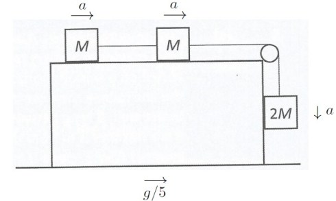
m/s placed on the block, are connected by a taut inextensible string. A second string passes over a light, smooth, fixed pulley to a third particle of mass
  which presses against the block as shown in the diagram.
 :
:


 and
and  they are calculated in MATH7021A1 – Student Data.
 ;
; 
 ;
;  ;
; 
 ;
; 
 ,
,  ,
,  ,
,  , approximate
  .
. ,
,  ,
,  , investigate the behaviour of
  for large
  .
. ,
,  ,
,  , run the Heun program. Comment on the behaviour of
  . Comment on the behaviour of
  ,
,  , run the Heun program. Comment on the behaviour of


Recent Comments