
You are currently browsing the category archive for the ‘Research’ category.
Taken from Random Walks on Finite Quantum Groups by Franz & Gohm.
The most important special case of the construction from here is obtained when we choose 


Suppose now that 
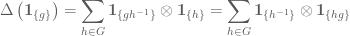
We also have

where ![[p(h,g)]](https://s0.wp.com/latex.php?latex=%5Bp%28h%2Cg%29%5D&bg=ffffff&fg=545454&s=0&c=20201002)
This calculation makes perfect sense when 

Now calculate

![\displaystyle[(I_{F(G)}\otimes T_\phi)\circ\Delta]\mathbf{1}_{\{g\}}=(I_{F(G)}\otimes T_\phi)\sum_{t\in G}\mathbf{1}_{\{t^{-1}\}}\otimes\mathbf{1}_{\{tg\}}](https://s0.wp.com/latex.php?latex=%5Cdisplaystyle%5B%28I_%7BF%28G%29%7D%5Cotimes+T_%5Cphi%29%5Ccirc%5CDelta%5D%5Cmathbf%7B1%7D_%7B%5C%7Bg%5C%7D%7D%3D%28I_%7BF%28G%29%7D%5Cotimes+T_%5Cphi%29%5Csum_%7Bt%5Cin+G%7D%5Cmathbf%7B1%7D_%7B%5C%7Bt%5E%7B-1%7D%5C%7D%7D%5Cotimes%5Cmathbf%7B1%7D_%7B%5C%7Btg%5C%7D%7D&bg=ffffff&fg=545454&s=0&c=20201002)

Now reindex the second sum here 


For random walks on a finite quantum groups there are some natural special choices for the initial distribution 


Inasmuch as I can tell, we have

On the other hand, stationarity of the random walk can be obtained if 

Proposition 4.1
The random walks on a finite quantum group are stationary for all choices of 
Proof : This follows from Proposition 3.2 together with the fact that the Haar state is characterised by its right invariance.
Taken from Condition Expectation in Quantum Probabilty by Denes Petz.
In quantum probability there are a number of fundamental questions that ask how faithfully can one quantise classical probability. Suppose that 


Suppose now that 

Taken from Real Analysis and Probability by R.M. Dudley.
For a sequence of 
The Cartesian product of finitely many 


For each 


Let 


Taken from C*-Algebras and Operator Theory by Gerald J. Murphy.
Although the principal aim of this section is to construct direct limits of C*-algebras, we begin with direct limits of groups.
If 


If 

If 


commutes for each 


The following runs a thread through what I’ve looked at over the past year: Progression Report.
Taken from Hopf Algebras by Abe. I am not doing this over a commutative ring as he is doing but just over the field of complex numbers, 
In this section the notion of algebras will be introduced; and we will present some examples of such algebras. An algebra over
Algebras
Suppose 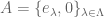


then 

From this fact, we see that an algebra

(the associative law)

(the unitary property)
Here, 

Taken from Hopf Algebras by Abe. This is not even nearly finished however I pressed publish instead of save draft… oh well.
In this section, we give the definition of Hopf algebras and present some examples. We begin by defining coalgebras, which are in a dual relationship with algebras., then bialgebras and Hopf algebras as algebraic systems in which the structures of algebras and coalgebras are interrelated by certain laws.
1.1 Coalgebras
We define a coalgebra dually to an algebra. Given an algebra 


(the coassociative law).

(the counitary property)
The maps 
Taken from C*-Algebras and Operator Theory by Gerald Murphy.
This section is concerned with positive linear functionals and representations. Pure states are introduced and shown to be the extreme points of a certain convex set, and their existence is deduced from the Krein-Milman theorem. From this the existence of irreducible representations is proved by establishing a correspondence between them and the pure states.
If 


We now return to the GNS construction associated to a state to show that the representations involved are cyclic.
Theorem 5.1.1
Let 


Moreover, 


Quantisation
I had been of the understanding that a quantisation looks as follows. There is some process or property 


Now from 
So essentially, this means that I thought you quantised objects, such as Markov chains, by replacing a commutative C*-algebra
Taken from Franz & Gohm.
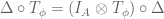
Let return to the map 


for all 


Recent Comments