You are currently browsing the category archive for the ‘General’ category.

TL;DR: The margin of error gets smaller with the proportion: the given margin of error is most relevant the closer to 50% the support.

Warning: I am taking the polls to be of the form

Will you vote for party X: yes or no?

There is more than a little confusion about the margin of error in political polling amongst the Irish political commentators.

Polls frequently come with margins of error such as “3%” and if a small party polls less than this some people comment that the real support could be zero.

In this piece, I will present a new way of interpreting low poll numbers, show how it is derived, further explain where the approximate 3% figure comes from and show what the calculation should be for mid-ranking proportions.

The main point is that none of these margins of error are accurate for small proportions.

For those who don’t like the mathematics of it all I will explain in a softer way why polling at 1-2% is very unlikely when your true support is 0.5%.

Read the rest of this entry »

The reality of the situation is that a far greater proportion than 5.2% of Leaving Cert students sitting Higher Level maths are presenting work that should confer less than 40% on their exam and those in the system know that the marking scheme receives a thorough massaging in order to get 94.8% of this cohort through.

A number of students are simply not allowed fail because failing 8-20+% of those sitting would be a political and logistical nightmare.

The final result of this fear of failing students, is the dumbing down of Higher Level maths and this is good for nobody.

I feel a solution to this is to do away with the pass/fail regime for maths: keep LC points for grades above 40% but mark the papers properly. This would effectively do away with the requirement for a pass in maths for third level courses, save for those such as engineering and science who want students with certain grades.

This will allow students take on Higher Level maths in good faith with the knowledge that if they do get less than 40%, it will not be a total disaster and they will still be able to attend a third level institution.

There is still a cut off in that 35% would confer 0 points and 40% would confer 70 points but this cut-off already exists (in theory!) but it is the failing not the lack of points that is somehow forcing the Department of Education to pass these students who really should be failing.

We should keep the bonus points for higher level maths because we should want our pupils to have good maths skills for the smart economy. However, at the moment, the stick of failing is proving to have more impact than the carrot of the 25 extra points.

I gave this talk at the CIT Spring Seminar Series.

This is about as short and introduction to quantum groups as you can imagine: I only had 15 minutes!

Let \mathbb{G} be a finite quantum group described by A=\mathcal{C}(\mathbb{G}) with an involutive antipode (I know this is true is the commutative or cocommutative case. I am not sure at this point how restrictive it is in general. The compact matrix quantum groups have this property so it isn’t a terrible restriction.) S^2=I_A. Under the assumption of finiteness, there is a unique Haar state, h:A\rightarrow \mathbb{C} on A.

Representation Theory

A representation of \mathbb{G} is a linear map \kappa:V\rightarrow V\otimes A that satisfies

\left(\kappa\otimes I_A\right)\circ\kappa =\left(I_V\otimes \Delta\right)\circ \kappa\text{\qquad and \qquad}\left(I_V\otimes\varepsilon\right)\circ \kappa=I_V.

The dimension of \kappa is given by \dim\,V. If V has basis \{e_i\} then we can define the matrix elements of \kappa by

\displaystyle\kappa\left(e_j\right)=\sum_i e_i\otimes\rho_{ij}.

One property of these that we will use it that \varepsilon\left(\rho_{ij}\right)=\delta_{i,j}.

Two representations \kappa_1:V_1\rightarrow V_1\otimes A and \kappa_2:V_2\rightarrow V_2\otimes A are said to be equivalent, \kappa_1\equiv \kappa_2, if there is an invertible intertwiner between them. An intertwiner between \kappa_1 and \kappa_2 is a map T\in L\left(V_1,V_2\right) such that

\displaystyle\kappa_2\circ T=\left(T\otimes I_A\right)\circ \kappa_1.

We can show that every representation is equivalent to a unitary representation.

Timmermann shows that if \{\kappa_\alpha\}_{\alpha} is a maximal family of pairwise inequivalent irreducible representation that \{\rho_{ij}^\alpha\}_{\alpha,i,j} is a basis of A. When we refer to “the matrix elements” we always refer to such a family. We define the span of \{\rho_{ij}\} as \mathcal{C}\left(\kappa\right), the space of matrix elements of \kappa.

Given a representation \kappa, we define its conjugate, \overline{\kappa}:\overline{V}\rightarrow\overline{V}\otimes A, where \overline{V} is the conjugate vector space of V, by

\displaystyle\overline{\kappa}\left(\bar{e_j}\right)=\sum_i \bar{e_i}\otimes\rho_{ij}^*,

so that the matrix elements of \overline{\kappa} are \{\rho_{ij}^*\}.

Timmermann shows that the matrix elements have the following orthogonality relations:

  • If \alpha and \beta are inequivalent then h\left(a^*b\right)=0, for all a\in \mathcal{C}\left(\kappa_\alpha\right) and b\in\mathcal{C}\left(\kappa_\beta\right).
  • If \kappa is such that the conjugate, \overline{\kappa}, is equivalent to a unitary matrix (this is the case in the finite dimensional case), then we have

\displaystyle h\left(\rho_{ij}^*\rho_{kl}\right)=\frac{\delta_{i,k}\delta_{j,l}}{d_\alpha}.

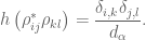
This second relation is more complicated without the S^2=I_A assumption and refers to the entries and trace of an intertwiner F from \kappa to the coreprepresention with matrix elements \{S^2\left(\rho_{ij}\right)\}. If S^2=I_A, then this intertwiner is simply the identity on V and so the the entries \left[F\right]_{ij}=\delta_{i,j} and the trace is d=\dim V.

Denote by \text{Irr}(\mathbb{G}) the set of unitary equivalence classes of irreducible unitary representations of \mathbb{G}. For each \alpha\in\text{Irr}(\mathbb{G}), let \kappa_\alpha:V_{\alpha}\rightarrow V_{\alpha}\otimes A be a representative of the class \alpha where V_\alpha is the finite dimensional vector space on which \kappa_\alpha acts.

Diaconis-Van Daele Fourier Theory

Read the rest of this entry »

I will be giving this talk with some of the fourth and fifth class pupils at Gaelscoil an Ghoirt Alainn, Mayfield in a few weeks.

A few historical and actual inaccuracies to keep things simple!

We define the transfer function of a black box model as

\displaystyle H(s)=\frac{Y(s)}{X(s)},

where X(s) is the Laplace transform of the input and Y(s) is the Laplace transform of the output. This yields:

Y(s)=H(s)\cdot X(s).

H(s) is a rational function and therefore has zeroes and roots (removable poles and roots are removed) and therefore so does Y(s):

\displaystyle Y(s)=K\cdot \frac{\prod_{j=1}^m(s-z_j)}{\prod_{i=1}^n(s-p_i)}.

These \{z_j\} are the zeroes of Y(s) and the \{p_i\} are the poles of Y(s)This means that we have (assuming m<n) a partial fraction expansion:

\displaystyle Y(s)=\sum_{i=1}^n\frac{C_i}{s-p_i}.

Applying the Inverse Laplace transform we have an input:

y(t)=\sum_{i=1}^n C_ie^{p_it}.

These p_i are complex numbers and depending on their nature we get different behaviours.

A positive real pole is a pole p\in\mathbb{R} such that p>0. This corresponds to an output e^{pt} which tends to infinity as t\rightarrow \infty. This is divergent or unstable behaviour.

A negative real pole p=-a with a>0 corresponds to an output \displaystyle e^{pt}=e^{-at}=\frac{1}{e^{at}}\rightarrow 0 as t\rightarrow \infty. This is convergent or stable behaviour.

A zero pole p=0 yields an output e^{pt}=e^{0\cdot t}=e^0=1 which is a constant output (which is considered stable).

A purely imaginary pole p=k i is, via Euler Formula, corresponds to oscillatory behaviour:

e^{pt}=e^{ikt}=\cos(kt)+i\sin(kt).

A genuinely complex pole p=a+ik (a>0) with a positive real part (in the right-half plane) corresponds to the following output

e^{pt}=e^{(a+ik)t}=e^{at+ikt}=e^{at}e^{ikt}=e^{at}(\cos(kt)+i\sin(kt)).

While the e^{ikt} component is oscillations, the e^{at} goes to zero so we get behaviour that looks like:

Graph

Note that this behaviour is unstable.

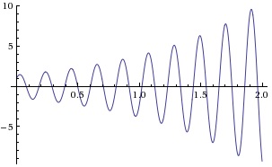
When we have complex pole p=-a+ik (a>0) with a strictly negative real part (a pole in the left-half plane), then we have e^{pt}=e^{-at}(\cos(kt)+i\sin(kt)). Note that we have oscillations but modulated by a decreasing e^{-at}. This is the motion of an underdamped harmonic oscillator:

Graph2

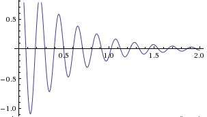
This is inherently stable behaviour.

This is the first in a series of posts that are an attempt by me to understand why my Industrial Measurement and Control students need to study the Laplace Transform.

Consider a black box model that takes as an input signal a function x(t) and produces an output signal y(t). For reasons that are as of yet not clear to me, we can take all of the derivatives of y(t) (and x(t)) to vanish for t=0.

Definition

The transfer function of a black box model is defined as

\displaystyle H(s)=\frac{Y(s)}{X(s)},

where Y(s) and X(s) are the Laplace Transforms of y(t) and x(t).

Note we have the Laplace transform of a function f(t) is a function F(s) defined by

F(s)=\mathcal{L}\{f(t)\}=\int_{0}^\infty f(t)e^{-st}\,dt.

Poles of H(s) are complex numbers z such that X(z)=0. For example, for an input signal x(t)=e^t, the transfer function has a pole at s=1 as

\displaystyle F(s)=\frac{1}{s-1}.

If the coefficients of x(t) are real, then in general the poles of the transfer are real or come in conjugate root pairs.

Read the rest of this entry »

I went through the first four weird facts from this talk with the some of the fifth and sixth class pupils at Gaelscoil an Ghoirt Alainn, Mayfield.

We have \sin^{2n}(x)+\cos^{2n}(x) has period \pi/2 for n\in\mathbb{N}\backslash \{1\}:


Also \sin^{2n+1}(x)+\cos^{2n+1}(x) has period 2\pi for n\in\mathbb{N}:


We have \sin^{-2n}(x)+\cos^{-2n}(x) has period \pi/2 for n\in\mathbb{N}:


Also \sin^{-2n+1}(x)+\cos^{-2n+1}(x) has period 2\pi for n\in\mathbb{N}:


Just a nice little problem I saw. The solution is not difficult but here I present a different one which I like.

Let \mathbb{P}_{1,001} be the vector space of polynomials of degree at most 1,000. Let T:\mathbb{P}_{1,001}\rightarrow \mathbb{P}_{1,001} be the linear map defined by:

\displaystyle T\{p(x)\}=2p'(x)-p(x).

Find the eigenvalues and eigenfunctions of the linear map T.

Read the rest of this entry »