Category Archive

You are currently browsing the category archive for the ‘General’ category.

On Parallel and Perpendicular Lines

June 5, 2018 in A1 Leaving Cert Maths, General, Grinds, Leaving Cert | Leave a comment

The purpose of this post is to briefly discuss parallelism and perpendicularity of lines in both a geometric and algebraic setting.

Lines

What is a line? In Euclidean Geometry we usually don’t define a line and instead call it a primitive object (the properties of lines are then determined by the axioms which refer to them). If instead points and line segments – defined by pairs of points $P,Q$ – $[PQ]$ are taken as the primitive objects, the following might define lines:

Geometric Definition Candidate

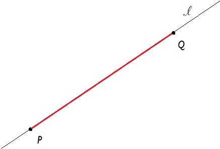
A line, $\ell$ , is a set of points with the property that for each pair of points in the line, $P,Q\in \ell$ ,

$[PQ]\cap \ell=[PQ]$ .

In terms of a picture this just says that when you have a line, that if you take two points in the line (the language in comes from set theory), that the line segment is a subset of the line:

line

Exercise:

Why is this objectively not a good definition of a line.

Once we move into Cartesian\Coordinate Geometry we can perhaps do a similar trick. We can use line segments, and their lengths to define slope, (slope = rise over run) and then define a line as follows:

Algebraic Definition Candidate

A line, $\ell$ , is a set of points such that for all pairs of distinct points $P,Q\in\ell$ , the slope is a constant.

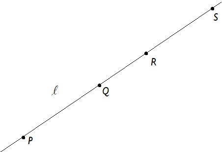
This means that if you take two pairs of distinct points in a line $\ell$ , and then calculate the slopes between them, you get the same answer, and therefore it makes sense to talk about the slope of a line, $m$ .

line2

This definition, however, has exactly the same problem as the previous. The definition we use isn’t too important but I do want to use a definition that considers the line a set of points.

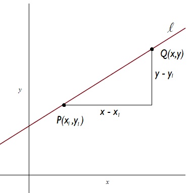
The Equation of a Line

We can use such a definition to derive the equation of a line ‘formula’ for a line of slope $m$ containing a point $(x_1,y_1)$ .

Suppose first of all that we have an $x\text{-}y$ axis and a point $P(x_1,y_1)$ in the line. What does it take for a second point $Q(x,y)$ to be in the line?

line4

Read the rest of this entry »

The Line of Best Fit

March 2, 2018 in A1 Leaving Cert Maths, Data Science, General, Leaving Cert, MATH6000, MATH7019 | Leave a comment

“Straight-Line-Graph-Through-The-Origin”

The words of Mr Michael Twomey, physics teacher, in Coláiste an Spioraid Naoimh, I can still hear them.

There were two main reasons to produce this straight-line-graph-through-the-origin:

to measure some quantity (e.g. acceleration due to gravity, speed of sound, etc.)
to demonstrate some law of nature (e.g. Newton’s Second Law, Ohm’s Law, etc.)

We were correct to draw this straight-line-graph-through-the origin for measurement, but not always, perhaps, in my opinion, for the demonstration of laws of nature.

The purpose of this piece is to explore this in detail.

Direct Proportion

Two variables $P$ and $Q$ are in direct proportion when there is some (real number) constant $k$ such that $P=k\cdot Q$ .

Read the rest of this entry »

Writing a Cosine Plus Sine as a Sine

January 29, 2018 in A1 Leaving Cert Maths, General, Grinds, Leaving Cert, Leaving Cert Applied Maths, MATH6014 | Leave a comment

Occasionally, it might be useful to do as the title here suggests.

Two examples that spring to mind include:

solving $a\cdot\cos\theta\pm b\cdot\sin\theta=c$ for $\theta$ (relative velocity example with $-$ below)
maximising $a\cdot\cos\theta\pm b\cdot\sin\theta$ without the use of calculus

$a\cdot \cos\theta- b\cdot\sin\theta$

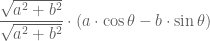
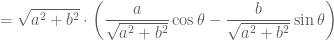
Note first of all the similarity between:

$\displaystyle a\cdot \cos\theta-b\cdot \sin \theta\sim \sin\phi\cos\theta-\cos\phi\sin\theta$ .

This identity is in the Department of Education formula booklet.

The only problem is that $a$ and $b$ are not necessarily sines and cosines respectively. Consider them, however, as opposites and adjacents to an angle in a right-angled-triangle as shown:

triangle

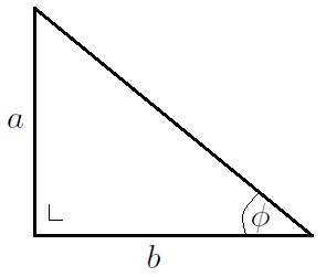
Using Pythagoras Theorem, the hypotenuse is $\sqrt{a^2+b^2}$ and so if we multiply our expression by $\displaystyle \frac{\sqrt{a^2+b^2}}{\sqrt{a^2+b^2}}$ then we have something:

$\displaystyle \frac{\sqrt{a^2+b^2}}{\sqrt{a^2+b^2}}\cdot \left(a\cdot \cos\theta- b\cdot\sin\theta\right)$

$\displaystyle=\sqrt{a^2+b^2}\cdot \left(\frac{a}{\sqrt{a^2+b^2}}\cos\theta-\frac{b}{\sqrt{a^2+b^2}}\sin\theta\right)$

$=\sqrt{a^2+b^2}\cdot \left(\sin\phi\cos\theta-\cos\phi\sin\theta\right)=\sqrt{a^2+b^2}\sin(\phi-\theta)$ .

Similarly, we have

$a\cdot\cos\theta+b\cdot \sin\theta=\sqrt{a^2+b^2}\sin(\phi+\theta)$ ,

where $\displaystyle\sin\phi=\frac{a}{\sqrt{a^2+b^2}}$ .

Read the rest of this entry »

A Two-Player Monty Hall Problem

January 26, 2018 in General | Leave a comment

Last semester, teaching some maths to engineers, I decided to play (via email) the Guess 2/3 of the Average game. Two players won (with guesses of 22) and so I needed a tie breaker.

I came up with a hybrid of Monty Hall, not too dissimilar to the game below (the prize was €5).

Rules

In this game, the host presents four doors to the players Alice and Bob:

monty

Behind three of the doors is an empty box, and behind one of the doors is €100.

The host flips a coin and asks the Alice would she like heads or tails. If she is correct, she gets to choose whether to go first or second.

The player that goes first picks a door, then the second player gets a turn, picking a different door.

Then the host opens a door revealing an empty box.

Now the first player has a choice to stay or switch.

The second player then has a choice to stay or switch (the second player can go to where the first player was if the first player switches).

Questions:

What is the best strategy for the player who goes second:
- if the first player switches?
- if the first player stays?
Should the person who wins the toss choose to go first or second? What assumptions did you make?
How much would you pay to play this game? What assumptions did you make?
If there is a bonus for playing second, how much should the bonus be such that the answer to question 1. is “it doesn’t matter”.

Correlation, Causation, and Ramsey Theory

January 25, 2018 in Data Science, General, MATH7019 | Leave a comment

Correlation does not imply causation is a mantra of modern data science. It is probably worthwhile at this point to define the terms correlation, imply, and (harder) causation.

Correlation

For the purposes of this piece, it is sufficient to say that if we measure and record values of variables $x$ and $y$ , and they appear to have a straight-line relationship, then the correlation is a measure of how close the data is to being on a straight line. For example, consider the following data:

graph14

The variables $y$ and $x$ have a strong correlation.

Causation

Causality is a deep philosophical notion, but, for the purposes of this piece, if there is a relationship between variables $y$ and $x$ such that for each value of $x$ there is a single value of $y$ , then we say that $y$ is a function of $x$ : $x$ is the cause and $y$ is the effect.

In this case, we write $y=f(x)$ , said $y$ is a function of $x$ . This is a causal relationship between $x$ and $y$ . (As an example which shows why this definition is only useful for the purposes of this piece, is the relationship between sales $t$ days after January 1, and the sales, $S$ , on that day: for each value of $t$ there is a single value of $S$ : indeed $S$ is a function of $t$ , but $t$ does not cause $S$ ).

Read the rest of this entry »

MATH6028: Chaos Theory II

November 21, 2017 in General, MATH6028, MS 3011 | Leave a comment

This follows on from this post.

Recall the Doubling Mapping $D:[0,1)\rightarrow [0,1)$ given by:

$\displaystyle D(x)=\begin{cases} 2x & \text{ if }x<1/2 \\ 2x-1 & \text{ if }x\geq 1/2 \end{cases}$

At the end of the last post we showed that this dynamical system displays sensitivity to initial conditions. Now we show that it displays topological mixing (a chaotic orbit) and density of periodic points.

First we must talk about periodic points.

Periodic Points

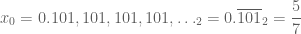
Consider, for example, the initial state $\displaystyle x_0=\frac{1}{9}$ . The orbit of $x_0$ is given by:

$\displaystyle \text{orb}(x_0)=\left\{\frac{1}{9},\frac29,\frac49,\frac89,\frac79,\frac59,\frac19,\frac29,\dots\right\}$

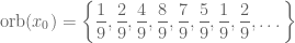
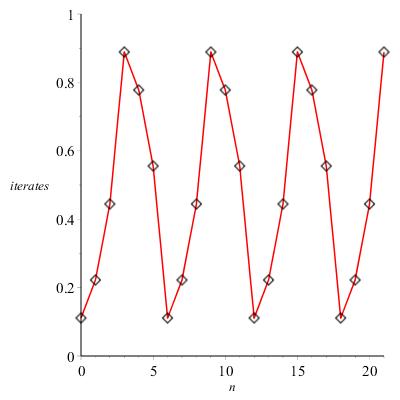
Here we see $\frac19$ repeats itself and so gets ‘stuck’ in a repeating pattern:

graph1

The orbit of $x_0=1/9$ .

The orbit of any fraction, e.g. $\displaystyle x_0=\frac{4}{243}$ , must be periodic, because $\displaystyle D\left(\frac{i}{243}\right)$ is either equal to $\displaystyle \frac{2i}{243}$ of $\displaystyle \frac{2i-243}{243}$ and so the orbit consists only of states of the form:

$\displaystyle \frac{i}{243}$ ,

and there are only 243 of these and so after 244 iterations, some state must be repeated and so we get locked into a periodic cycle.

If we accept the following:

Proposition

A fraction $\frac{p}{q}$ has a recurring binary expansion:

$\displaystyle \frac{p}{q}=0.b_1\dots b_m\overline{a_1a_2\dots a_n}_2$ ,

then this is another way to see that fractions are (eventually) periodic. Take for example,

$\displaystyle x_0=0.101,101,101,101,\dots_2=0.\overline{101}_2=\frac{5}{7}$ .

Read the rest of this entry »

MATH6028: Chaos Theory (Part I)

November 14, 2017 in General, MATH6028, MS 3011 | 1 comment

Dynamical Systems

A dynamical system is a set of states $S$ together with an iterator function $f:S\rightarrow S$ which is used to determine the next state of a system in terms of the previous state. For example, if $x_0\in S$ is the initial state, the subsequent states are given by:

$x_1=f(x_0)$ ,

$x_2=f(x_1)=f(f(x_0))=(f\circ f)(x_0)=:f^2(x_0)$

$x_3=f(x_2)=f(f^2(x_0))=f^3(x_0)$ ,

and in general, the next state is got by applying the iterator function:

$x_{i}=f(x_{i-1})=f^i(x_0)$ .

The sequence of states

$\{x_0,x_1,x_2,\dots\}$

is known as the orbit of $x_0$ and the $x_i$ are known as the iterates.

Such dynamical systems are completely deterministic: if you know the state at any time you know it at all subsequent times. Also, if a state is repeated, for example:

$\text{orb}(x_0)=\{x_0,x_1,x_2,x_3,x_4=x_2,x_5\dots,\}$

then the orbit is destined to repeated forever because

$x_5=f(x_4)=f(x_2)=x_3$ ,

$x_6=f(x_5)=f(x_3)=x_4=x_2$ , etc:

$\Rightarrow \text{orb}(x_0)=\{x_0,x_1,x_2,x_3,x_2,x_3,x_2,\dots\}$

Example: Savings

Suppose you save in a bank, where monthly you receive $0.1\%=0.001$ interest and you throw in $50$ per month, starting on the day you open the account.

This can be modeled as a dynamical system.

Let $S=\mathbb{R}$ be the set of euro amounts. The initial amount of savings is $x_0=50$ . After one month you get interest on this: $0.001\times50$ , you still have your original $50$ and you are depositing a further €50, so the state of your savings, after one month, is given by:

$x_1=50+0.001\times 50+50=(1+0.001)50+50$ .

Now, in the second month, there is interest on all this:

interest in second month $0.001\times((1+0.001)50+50)=0.001x_1$ ,

we also have the $x_1=(1+0.001)50+50$ from the previous month and we are throwing in an extra €50 so now the state of your savings, after two months, is:

$x_2=x_1+0.001x_1+50=(1+0.001)x_1+50$ ,

and it shouldn’t be too difficult to see that how you get from $x_i\longrightarrow x_{i+1}$ is by applying the function:

$f(x)=(1+0.001)x+50$ .

Exercise

Use geometric series to find a formula for $x_n$ .

Weather

If quantum effects are neglected, then weather is a deterministic system. This means that if we know the exact state of the weather at a certain instant (we can even think of the state of the universe – variations in the sun affecting the weather, etc), then we can calculate the state of the weather at all subsequent times.

This means that if we know everything about the state of the weather today at 12 noon, then we know what the weather will be at 12 noon tomorrow…

Read the rest of this entry »

How does a Curve have an Equation?

November 1, 2017 in A1 Leaving Cert Maths, General, MATH6015, MATH6040, MATH6055 | 8 comments

In school, we learn how a line has an equation… and a circle has an equation… what does this mean?

The short answer is

points $(x_0,y_0)$ on curve $\longleftrightarrow$ solutions $(x_0,y_0)$ of equation

however this note explains all of this from first principles, with a particular emphasis on the set-theoretic fundamentals.

Set Theory

A set is a collection of objects. The objects of a set are referred to as the elements or members and if we can list the elements we include them in curly-brackets. For example, call by $S$ the set of whole numbers (strictly) between two and nine. This set is denoted by

$S=\{3,4,5,6,7,8\}$ .

We indicate that an object $x$ is an element of a set $X$ by writing $x\in X$ , said, $x$ in $X$ or $x$ is an element of $X$ . We use the symbol $\not\in$ to indicate non-membership. For example, $2\not\in S$ .

Elements are not duplicated and the order doesn’t matter. For example:

$\{x,x,y\}=\{x,y\}=\{y,x\}$ .

Read the rest of this entry »

Solving ‘Easy’ Equations: Part II

October 12, 2017 in A1 Leaving Cert Maths, General, Grinds, Leaving Cert | Leave a comment

This post follows on from this post where the following principle was presented:

Fundamental Principle of Solving ‘Easy’ Equations

Identify what is difficult or troublesome about the equation and get rid of it. As long as you do the same thing to both numbers (the “Lhs” and the “Rhs”), the equation will be replaced by a simpler equation with the same solution.

There are a number of subtleties here: basically sometimes you get extra ‘solutions’ (that are not solutions at all), and sometimes you can lose solutions.

Let us write the squaring function, e.g. $6\mapsto 36$ , $x\mapsto x^2$ by $f(x)=x^2$ and the square-rooting function by $x\mapsto \sqrt{x}$ . It appears that $(x^2,\sqrt{x})$ are an inverse pair but not quite exactly. While

$\displaystyle 81\overset{\sqrt{x}}{\mapsto} 9\overset{x^2}{\mapsto}81$ and

$\displaystyle 7\overset{x^2}{\mapsto}49\overset{\sqrt{x}}{\mapsto}7$ ,

check out O.K. note that

$-4\overset{x^2}{\mapsto}+16\overset{\sqrt{x}}{\mapsto}=+4\neq -4$ ,

does not bring us back to where we started.

This problem can be fixed by restricting the allowable inputs to $x^2$ to positive numbers only but for the moment it is better to just treat this as a subtlety, namely while $(\sqrt{x})^2=x$ , $\sqrt{x^2}=\pm x$ … in fact I recommend that we remember that with an $x^2$ there will generally be two solutions.

The other thing we look out for as much as possible is that we cannot divide by zero.

There are other issues around such as the fact that $\sqrt{x}>0$ , so that the equation $\sqrt{x}=-2$ has no solutions (no, $x=4$ is not a solution! Check.). This equation has no solutions.

Often, in context, these subtleties are not problematic. For example, equations with no solutions rarely arise and quantities might be positive so that if we have $\pm\sqrt{a}$ , only $+\sqrt{a}$ need be considered (for example, $a$ might be a length).

Read the rest of this entry »

Why Do We Multiply Matrices Like We Do?

September 29, 2017 in General, MATH6040, MATH8009 | 6 comments

In this short note we will explain why we multiply matrices in this “rows-by-columns” fashion. This note will only look at $2\times 2$ matrices but it should be clear, particularly by looking at this note, how this generalises to matrices of arbitrary size.

First of all we need some objects. Consider the plane $\Pi$ . By fixing an origin, orientation ( $x$ – and $y$ -directions), and scale, each point $P\in\Pi$ can be associated with an ordered pair $(a,b)$ , where $a$ is the distance along the $x$ axis and $b$ is the distance along the $y$ axis. For the purposes of linear algebra we denote this point $P=(a,b)$ by

$\displaystyle P=\left(\begin{array}{c}a\\ b\end{array}\right)$ .

graph7

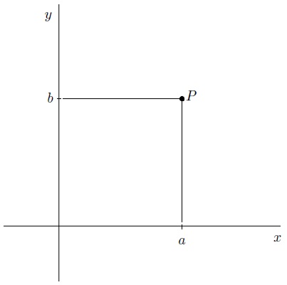
We have two basic operations with points in the plane. We can add them together and we can scalar multiply them according to, if $Q=(c,d)$ and $\lambda\in\mathbb{R}$ :

$P+Q=\left(\begin{array}{c}a\\ b\end{array}\right)+\left(\begin{array}{c}c\\ d\end{array}\right)$

$\displaystyle=\left(\begin{array}{c}a+c\\ b+d\end{array}\right)$ , and

$\lambda\cdot P=\lambda\cdot \left(\begin{array}{c}a\\ b\end{array}\right)=\left(\begin{array}{c}\lambda\cdot a\\ \lambda\cdot b\end{array}\right)$ .

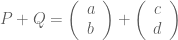
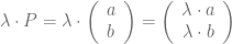
Objects in mathematics that can be added together and scalar-multiplied are said to be vectors. Sets of vectors are known as vector spaces and a feature of vector spaces is that all vectors can be written in a unique way as a sum of basic vectors.

Read the rest of this entry »

	J.P. McCarthy on MATH6040: Spring 2022, Week…
	J.P. McCarthy on MATH6040: Spring 2022, Week…
	J.P. McCarthy on MATH7019: Winter 2020, Week…
	J.P. McCarthy on MATH7019: Winter 2020, Week…
	A Sufficient Conditi… on Almost All Trees have Quantum…

Category Archive

On Parallel and Perpendicular Lines

Lines

Exercise:

The Equation of a Line

The Line of Best Fit

Direct Proportion

Writing a Cosine Plus Sine as a Sine

$a\cdot \cos\theta- b\cdot\sin\theta$

A Two-Player Monty Hall Problem

Rules

Correlation, Causation, and Ramsey Theory

Correlation

Causation

MATH6028: Chaos Theory II

Periodic Points

Proposition

MATH6028: Chaos Theory (Part I)

Dynamical Systems

Example: Savings

Exercise

Weather

How does a Curve have an Equation?

Set Theory

Solving ‘Easy’ Equations: Part II

Why Do We Multiply Matrices Like We Do?

Recent Comments

Categories

J.P. McCarthy Maths

Category Archive

Lines

Exercise:

The Equation of a Line

Share this:

Direct Proportion

Share this:

Share this:

Rules

Share this:

Correlation

Causation

Share this:

Periodic Points

Proposition

Share this:

Dynamical Systems

Example: Savings

Exercise

Weather

Share this:

Set Theory

Share this:

Share this:

Share this:

Recent Comments

Categories